Julia for Numerical Computation in MIT Courses

Several MIT courses involving numerical computation, including 18.06, 18.303, 18.330, 18.335/6.337, 18.337/6.338, and 18.338, are beginning to use Julia, a fairly new language for technical computing. This page is intended to supplement the Julia documentation with some simple tutorials on installing and using Julia targeted at MIT students. See also our Julia cheatsheet listing a few basic commands, and various Julia tutorials online.

In particular, we will be using Julia in the IJulia browser-based enviroment, which leverages your web browser and Jupyter to provide a rich environment combining code, graphics, formatted text, and even equations, with sophisticated plots via Matplotlib.

You can also look at the Jupyter notebook from the fall 2020 tutorial, as well as the tutorial video (MIT only).

Why Julia?

Julia is relatively new high-level free/open-source language for numerical computing in the same spirit, with a rich set of built-in types and libraries for working with linear algebra and other types of computations, with a syntax that is superficially reminiscent of Matlab's. Basically, we are using Julia because, unlike Matlab or Python or R, it scales better to real computational problems — you can write performance-critical "inner loops" in Julia, whereas similar tasks in other high-level languages often require one to drop down to C or similar low-level languages. (See e.g. this 6.172 lecture on performance in Julia vs. Python.) Because of this, we are using Julia more and more in our own research, and we want to teach using software tools that we really employ ourselves.

Running Julia in the cloud

The easiest way to get started with Julia is to run it in the cloud on mybinder.org, which is as easy as clicking this link:

That link opens up a default MIT-math Julia + Python environment that we set up, but you can also easily set up your own environments. Although the link above gives you access to our tutorial notebook here, you can create alternate links (e.g. for particular MIT courses) using nbgitpuller.

There are two major drawbacks to using the free mybinder.org service:

It's often slow (sometimes an order of magnitude slower than a typical laptop), especially to start up, although it's probably fast enough for simple problems in coursework.
It has a very short timeout: if you go for a coffee break, your session will probably have stopped running by the time you get back. Fortunately, there are save/download buttons that still work in a timed-out session, so you can save your work and restore it after restarting the binder session.
There are at most 100 simultaneous users for a given configuration repository. (Therefore, if your instructor wants to use mybinder for a course, encourage them to set up their own docker configuration, perhaps by forking our repo.)

Eventually you'll probably want to install Julia on your own computer to eliminate these frustrations. Fortunately, this is usually relatively easy:

Installing Julia and IJulia on your own computer

First, download the 1.6 release of Julia run the installer. Then run the Julia application (double-click on it); a window with a julia> prompt will appear. At the julia> prompt, type a ] (close square bracket) to get a Julia package prompt pkg>, where you can type

(v1.6) pkg> add IJulia

You may also want to install these packages, which we tend to use in a lot of the lecture materials:

(v1.6) pkg> add Interact PyPlot Plots

(You can install packages later as you need them using the same interface, of course. Thousands of other packages can be found on JuliaHub.)

Switch back to the julia> prompt by hitting backspace or ctrl-C, and then you can launch the notebook by running

julia> using IJulia

julia> notebook()

as is also described below.

(An alternative is to download the JuliaPro package, which includes Julia, IJulia, the Juno IDE based on the Atom editor, and a number of packages pre-installed.)

Troubleshooting:

If you ran into a problem with the above steps, after fixing the problem you can type build at the pkg> prompt to try to rerun the install scripts.
If you tried it a while ago, try running update at the pkg> prompt and try again: this will fetch the latest versions of the Julia packages in case the problem you saw was fixed. Run build IJulia at the pkg> prompt if your Julia version may have changed. If this doesn't work, try just deleting the whole .julia directory in your home directory (on Windows, it is called AppData\Roaming\julia\packages in your home directory) and re-adding the packages.
On MacOS, you need MacOS 10.8 or later.
If the notebook opens up, but doesn't respond (the input label is In[*] indefinitely), try creating a new Python notebook (not Julia) from the New button in the Jupyter dashboard, to see if 1+1 works in Python. If it is the same problem, then probably you have a firewall running on your machine (this is common on Windows) and you need to disable the firewall or at least to allow the IP address 127.0.0.1. (For the Sophos endpoint security software, go to "Configure Anti-Virus and HIPS", select "Authorization" and then "Websites", and add 127.0.0.1 to "Authorized websites"; finally, restart your computer.)

Other Julia environments

Pluto.jl

A different interactive-computing environment for Julia is Pluto.jl, which runs in the browser like Jupyter but is more oriented towards "live" interaction where updating one piece of code automatically re-runs anything affected by that change. Running Julia is as easy as:

pkg> add Pluto

julia> using Pluto

julia> Pluto.run()

VSCode

For writing larger programs, modules, and packages (as opposed to little interactive snippets), you'll want to start putting code into files and modules, and use a more full-featured code-editing environment. A popular choice is the free/cross-platform Visual Studio Code (VSCode) editor, which has a Julia VSCode plugin to provide a full-featured integrated development environment (IDE).

Other Editors

Of course, there is also good support for editing Julia in many other programs, such as Emacs, Vim, Atom, and so forth.

Updating Julia and IJulia

Julia is improving rapidly, so it won't be long before you want to update to a more recent version. The same is true of Julia add-on packages like PyPlot. To update the packages only, keeping Julia itself the same, just run:

(v1.3) pkg> update

at the Julia pkg> prompt after typing ]; you can also run ] update in IJulia.

If you download and install a new version of Julia from the Julia web site, you will also probably want to update the packages with update (in case newer versions of the packages are required for the most recent Julia). In any case, if you install a new Julia binary (or do anything that changes the location of Julia on your computer), you must update the IJulia installation (to tell IPython where to find the new Julia) by running build at the Julia pkg> prompt line (not in IJulia).

Running Julia in the IJulia Notebook

Once you have followed the installation steps above, open up the Julia command line (run julia or double-click the julia program) and run

julia> using IJulia
julia> notebook()

(You will have to leave the Julia command-line window open in order to keep the IJulia/Jupyter process running. Alternatively, you can run notebook(detached=true) if you want to run the Jupyter server as a background process, at which point you can close the Julia command line, but then if you ever want to restart the Jupyter server you will need to kill it manually.

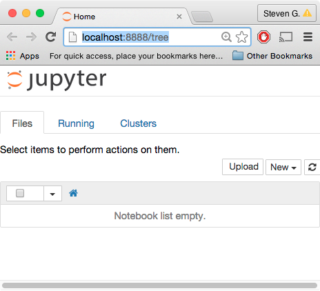
A "dashboard" window like this should open in your web browser (at address localhost:8888, which you can return to at any time as long as the notebook() server is running; I usually keep it running all the time):

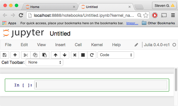
Now, click on the New button and select the Julia option to start a new "notebook". A notebook will combine code, computed results, formatted text, and images; for example, you might use one notebook for each problem set. The notebook window that opens will look something like:

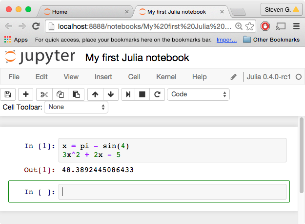
You can click the "Untitled" at the top to change the name, e.g. to "My first Julia notebook". You can enter Julia code at the In[ ] prompt, and hit shift-return to execute it and see the results. If you hit return without the shift key, it will add additional lines to a single input cell. For example, we can define a variable x (using the built-in constant pi and the built-in function sin), and then evaluate a polynomial 3x^2 + 2x - 5 in terms of x (note that, unlike Matlab or Python, we don't have to type 3*x^2 if we don't want to: a number followed by a variable is automatically interpreted as multiplication without having to type *):

The result that is printed (in Out[1]) is the last expression from the input cell, i.e. the polynomial. If you want to see the value of x, for example, you could simply type x at the second In[ ] prompt and hit shift-return.

See, for example, the mathematical operations in the Julia manual for many more basic math functions.

Plotting

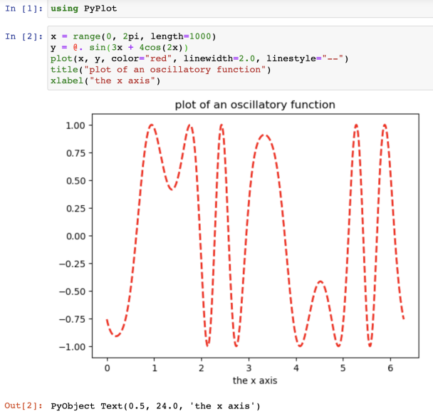
There are several plotting packages available for Julia. If you followed the installation instructions, above, you already have one full-featured Matlab-like plotting package installed: PyPlot, which is simply a wrapper around Python's amazing Matplotlib library.

To start using PyPlot to make plots in Julia, first type using PyPlot at an input prompt and hit shift-enter. using is the Julia command to load an external module (which must usually be installed first, e.g. by the ] add PyPlot command from the installation instructions above). The very first time you do using PyPlot, it will take some time: the module and its dependencies will be "precompiled" so that in subsequent Julia sessions it will load quickly.

Then, you can type any of the commands from Matplotlib, which includes equivalents for most of the Matlab plotting functions. For example:

Printing/exporting Notebooks

Currently, printing a notebook from the browser's Print command can be somewhat problematic. There are four solutions:

At the top of the notebook, click on the File menu (in the notebook, not the browser's global menu bar), and choose Print Preview. This should open up a window/tab that you can print normally.
For turning in homework, a class may allow you to submit the notebook file (.ipynb file) electronically (the graders will handle printing). You can save a notebook file in a different location by choosing Download as from the notebook's File menu.
The highest-quality printed output is produced by IPython's nbconvert utility. For example, if you have a file mynotebook.ipynb, you can run ipython nbconvert mynotebook.ipynb to convert it to an HTML file that you can open and print in your web browser. This requires you to install IPython, Sphinx (which is automatically installed with the Anaconda Python/IPython distribution), and Pandoc on your computer.
If you post your notebook in a Dropbox account or in some other web-accessible location, you can paste the URL into the online nbviewer to get a printable version.

Leon-Zhaohw/julia-mit