On the Error Analysis of 3D Gaussian Splatting and an Optimal Projection Strategy

ECCV 2024

Letian Huang Jiayang Bai Jie Guo^* Yuanqi Li Yanwen Guo
Nanjing University

News

[2024.11.14] 🖊️ Add derivation of the backward passes.

[2024.07.16] 🎈 We release the code.

[2024.07.05] Birthday of the repository.

TODO List

Release the code (submodule for the pinhole camera's rasterization).
Release the submodule for the panorama's rasterization.
Release the submodule for the fisheye camera's rasterization.
Code optimization (as mentioned in the limitation of the paper, the current CUDA implementation is slow and needs optimization).

Motivation

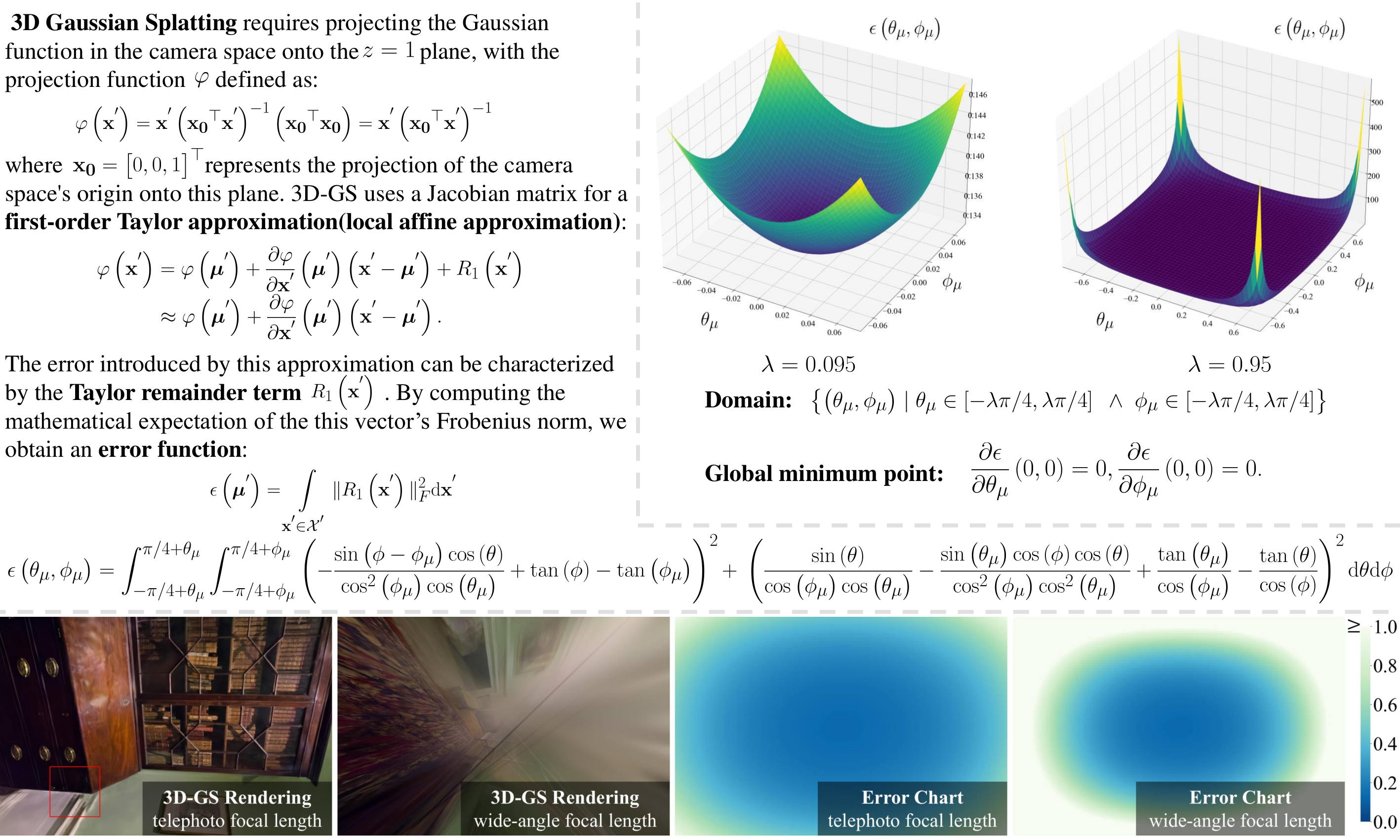
We derive the mathematical expectation of the projection error (Top left), visualize the graph of the error function under two distinct domains and analyze when this function takes extrema through methods of function optimization (Top right). We further derive the projection error function with respect to image coordinates and focal length through the coordinate transformation between image coordinates and polar coordinates and visualize this function, with the left-to-right sequence corresponding to the 3D-GS rendered images under long focal length, 3D-GS rendered images under short focal length, the error function under long focal length, and the error function under short focal length (Below).

Pipeline

Illustration of the rendering pipeline for our Optimal Gaussian Splatting and the projection of 3D Gaussian Splatting. The blue box depicts the projection process of the original 3D-GS, which straightforwardly projects all Gaussians onto the same projection plane. In contrast, the red box illustrates our approach, where we project individual Gaussians onto corresponding tangent planes.

Installation

Clone the repository and create an anaconda environment using

git clone git@github.com:LetianHuang/op43dgs.git
cd op43dgs

SET DISTUTILS_USE_SDK=1 # Windows only
conda env create --file environment.yml
conda activate op43dgs

The repository contains several submodules, thus please check it out with

# Pinhole
pip install submodules/diff-gaussian-rasterization-pinhole

# Panorama
pip install submodules/diff-gaussian-rasterization-panorama

# Fisheye
pip install submodules/diff-gaussian-rasterization-fisheye

Dataset

Mip-NeRF 360 Dataset

Please download the data from the Mip-NeRF 360.

Tanks & Temples dataset

Please download the data from the 3D Gaussian Splatting.

Deep Blending

Please download the data from the 3D Gaussian Splatting.

Training and Evaluation

By default, the trained models use all available images in the dataset. To train them while withholding a test set for evaluation, use the --eval flag. This way, you can render training/test sets and produce error metrics as follows:

python train.py -s <path to COLMAP or NeRF Synthetic dataset> --eval # Train with train/test split
python render.py -m <path to trained model> --fov_ratio 1 # Generate renderings

Command Line Arguments for render.py

--model_path / -m

Path to the trained model directory you want to create renderings for.

--skip_train

Flag to skip rendering the training set.

--skip_test

Flag to skip rendering the test set.

--quiet

Flag to omit any text written to standard out pipe.

--fov_ratio

Focal length reduction ratios.

Acknowledgements

This project is built upon 3DGS. Please follow the license of 3DGS. We thank all the authors for their great work and repos.

Citation

If you find this work useful in your research, please cite:

@inproceedings{10.1007/978-3-031-72643-9_15,
    author="Huang, Letian and Bai, Jiayang and Guo, Jie and Li, Yuanqi and Guo, Yanwen",
    title="On the Error Analysis of 3D Gaussian Splatting and an Optimal Projection Strategy",
    booktitle="Computer Vision -- ECCV 2024",
    year="2025",
    publisher="Springer Nature Switzerland",
    address="Cham",
    pages="247--263",
    isbn="978-3-031-72643-9"
}

Derivation in diff-gaussian-rasterization

About gradients of Gaussian's position

Given:

Gaussian's position in image space: $u, v$

Projection coordinates of the pixel on the unit sphere (in renderCUDA): $t_x, t_y, t_z$

Camera intrinsic parameters for pinhole: $f_x, f_y, c_x, c_y$

Forward

For the pinhole camera model, we can compute the corresponding camera coordinate based on the Gaussian position $u, v$ in image space:

$$ r_x = (u - c_x) / f_x, $$

$$ r_y = (v - c_y) / f_y, $$

$$ r_z = 1. $$

Then calculate the projection of $[r_x, r_y, r_z]^{\top}$ on the unit sphere:

$$ \mu_x = \frac{r_{x}}{\sqrt{r_{x}^{2} + r_{y}^{2} + r_{z}^{2}}}, $$

$$ \mu_y = \frac{r_{y}}{\sqrt{r_{x}^{2} + r_{y}^{2} + r_{z}^{2}}}, $$

$$ \mu_z = \frac{r_{z}}{\sqrt{r_{x}^{2} + r_{y}^{2} + r_{z}^{2}}}, $$

Subsequently, calculate the projection of $[t_x, t_y, t_z]^{\top}$ on the tangent plane $\mu_x x+\mu_y y+\mu_z z = 1$ :

$$ \mathbf{x}_{2D}=\begin{bmatrix} \frac{t_x}{\mu_x t_x + \mu_y t_y + \mu_z t_z} \newline \frac{t_y}{\mu_x t_x + \mu_y t_y + \mu_z t_z} \newline \frac{t_z}{\mu_x t_x + \mu_y t_y + \mu_z t_z} \end{bmatrix} $$

Then, calculate the matrix $\mathbf{Q}$ based on Equation 18 in the paper:

$$ \mathbf{Q}=\begin{bmatrix} \frac{\mu_{z}}{\sqrt{\mu_{x}^{2} + \mu_{z}^{2}}} & 0 & - \frac{\mu_{x}}{\sqrt{\mu_{x}^{2} + \mu_{z}^{2}}} \newline - \frac{\mu_{x} \mu_{y}}{\sqrt{\mu_{x}^{2} + \mu_{z}^{2}} \sqrt{\mu_{x}^{2} + \mu_{y}^{2} + \mu_{z}^{2}}} & \frac{\sqrt{\mu_{x}^{2} + \mu_{z}^{2}}}{\sqrt{\mu_{x}^{2} + \mu_{y}^{2} + \mu_{z}^{2}}} & - \frac{\mu_{y} \mu_{z}}{\sqrt{\mu_{x}^{2} + \mu_{z}^{2}} \sqrt{\mu_{x}^{2} + \mu_{y}^{2} + \mu_{z}^{2}}} \newline \frac{\mu_{x}}{\sqrt{\mu_{x}^{2} + \mu_{y}^{2} + \mu_{z}^{2}}} & \frac{\mu_{y}}{\sqrt{\mu_{x}^{2} + \mu_{y}^{2} + \mu_{z}^{2}}} & \frac{\mu_{z}}{\sqrt{\mu_{x}^{2} + \mu_{y}^{2} + \mu_{z}^{2}}}\end{bmatrix}\text{.} $$

Subsequently, the projection of the pixel onto the tangent plane after transformerd into the local coordinate system can be obtained through the $\mathbf{Q}$ matrix (The origin of the local coordinate system is the projection of the Gaussian mean onto the tangent plane):

$$ \begin{bmatrix} u_{pixf} \newline v_{pixf} \newline 1 \end{bmatrix}=\mathbf{Q}\mathbf{x}_{2D} $$

$$ =\begin{bmatrix}\frac{- \mu_{x} t_{z} + \mu_{z} t_{x}}{\sqrt{\mu_{x}^{2} + \mu_{z}^{2}} \left(\mu_{x} t_{x} + \mu_{y} t_{y} + \mu_{z} t_{z}\right)} \newline \frac{- \mu_{y} \left(\mu_{x} t_{x} + \mu_{z} t_{z}\right) + t_{y} \left(\mu_{x}^{2} + \mu_{z}^{2}\right)}{\sqrt{\mu_{x}^{2} + \mu_{z}^{2}} \sqrt{\mu_{x}^{2} + \mu_{y}^{2} + \mu_{z}^{2}} \left(\mu_{x} t_{x} + \mu_{y} t_{y} + \mu_{z} t_{z}\right)} \newline 1\end{bmatrix}. $$

Finally, the difference between the projection of the Gaussian mean and the pixel projection onto the tangent plane can be calculated:

$$ d_x = -u_{pixf},\quad d_y = -v_{pixf} $$

Backward

It is recommended to use scientific computing tools to compute the gradient!

First, calculate the partial derivatives of $d_x, d_y$ with respect to $r_x, r_y$:

$$ \frac{\partial d_x}{\partial r_x}=\frac{\partial d_x}{\partial \mu_x}\frac{\partial \mu_x}{\partial r_x}+\frac{\partial d_x}{\partial \mu_y}\frac{\partial \mu_x}{\partial r_x}+\frac{\partial d_x}{\partial \mu_z}\frac{\partial \mu_z}{\partial r_x},\quad \frac{\partial d_x}{\partial r_y}=\frac{\partial d_x}{\partial \mu_x}\frac{\partial \mu_x}{\partial r_y}+\frac{\partial d_x}{\partial \mu_y}\frac{\partial \mu_x}{\partial r_y}+\frac{\partial d_x}{\partial \mu_z}\frac{\partial \mu_z}{\partial r_y}, $$

$$ \frac{\partial d_y}{\partial r_x}=\frac{\partial d_y}{\partial \mu_x}\frac{\partial \mu_x}{\partial r_x}+\frac{\partial d_y}{\partial \mu_y}\frac{\partial \mu_x}{\partial r_x}+\frac{\partial d_y}{\partial \mu_z}\frac{\partial \mu_z}{\partial r_x},\quad \frac{\partial d_y}{\partial r_y}=\frac{\partial d_y}{\partial \mu_x}\frac{\partial \mu_x}{\partial r_y}+\frac{\partial d_y}{\partial \mu_y}\frac{\partial \mu_x}{\partial r_y}+\frac{\partial d_y}{\partial \mu_z}\frac{\partial \mu_z}{\partial r_y}. $$

Then, calculate the gradient of $r_x, r_y$ with respect to $u, v$ (gradients related to the camera model):

$$ \frac{\partial r_x}{\partial u}=1 / f_x,\quad \frac{\partial r_y}{\partial v}=1 / f_y. $$

Using the chain rule, we can obtain:

$$ \frac{\partial d_x}{\partial u}=\frac{\partial d_x}{\partial r_x}\frac{\partial r_x}{\partial u}, \quad \frac{\partial d_x}{\partial v}=\frac{\partial d_x}{\partial r_y}\frac{\partial r_y}{\partial v}, $$

$$ \frac{\partial d_y}{\partial u}=\frac{\partial d_y}{\partial r_x}\frac{\partial r_x}{\partial u}, \quad \frac{\partial d_y}{\partial v}=\frac{\partial d_y}{\partial r_y}\frac{\partial r_y}{\partial v}. $$