Author: Gabriel Espinola Lincoln Ferreira dos Santos
Heart failure (HF), also known as congestive heart failure (CHF), decompensatio cordis (DC), and congestive cardiac failure (CCF), is when the heart is unable to pump sufficiently to maintain blood flow to meet the body's needs. The study intend to do statistical analysis for heart failure in a dataset contains 12 features that can be used to predict mortality and correlating with articles.
Definition of done: Create a model for predicting mortality caused by Heart Failure.
Reference: Accessed by Capes periodicos
-
MCMURRAY,John; PONIKOWSKI,Piotr. Heart Failure Not Enough Pump Iron? Glasgow, Scotland, United Kingdom and Wroclaw, Poland
-
AM,Heart J Clinical predictors of heart failure in patients with first acute myocardial infarction
-
ALI,Abbas S.;Clinical predictors of heart failure in patients with first acute myocardial infarction
-
GOMES,Marilia B Impact of Diabetes on Cardiovascular Disease: An Update
-
Creatine phosphokinase test: https://www.mountsinai.org/health-library/tests/creatine-phosphokinase-test
-
Mohammed W. Akhter; Effect of Elevated Admission Serum Creatinine and Its Worsening on Outcome in Hospitalized Patients With Decompensated Heart Failure negrito
-
Matheus, Alessandra; Impact of Diabetes on Cardiovascular Disease: An Update
-
Abbas S. Ali; Clinical predictors of heart failure in patients with first acute myocardial infarction
import pandas as pd
import matplotlib.pyplot as plt
import seaborn as sns
df = pd.read_csv('Dataset.csv')
df.head(15).dataframe tbody tr th {
vertical-align: top;
}
.dataframe thead th {
text-align: right;
}
| age | anaemia | creatinine_phosphokinase | diabetes | ejection_fraction | high_blood_pressure | platelets | serum_creatinine | serum_sodium | sex | smoking | time | DEATH_EVENT | |
|---|---|---|---|---|---|---|---|---|---|---|---|---|---|
| 0 | 75.0 | 0 | 582 | 0 | 20 | 1 | 265000.00 | 1.9 | 130 | 1 | 0 | 4 | 1 |
| 1 | 55.0 | 0 | 7861 | 0 | 38 | 0 | 263358.03 | 1.1 | 136 | 1 | 0 | 6 | 1 |
| 2 | 65.0 | 0 | 146 | 0 | 20 | 0 | 162000.00 | 1.3 | 129 | 1 | 1 | 7 | 1 |
| 3 | 50.0 | 1 | 111 | 0 | 20 | 0 | 210000.00 | 1.9 | 137 | 1 | 0 | 7 | 1 |
| 4 | 65.0 | 1 | 160 | 1 | 20 | 0 | 327000.00 | 2.7 | 116 | 0 | 0 | 8 | 1 |
| 5 | 90.0 | 1 | 47 | 0 | 40 | 1 | 204000.00 | 2.1 | 132 | 1 | 1 | 8 | 1 |
| 6 | 75.0 | 1 | 246 | 0 | 15 | 0 | 127000.00 | 1.2 | 137 | 1 | 0 | 10 | 1 |
| 7 | 60.0 | 1 | 315 | 1 | 60 | 0 | 454000.00 | 1.1 | 131 | 1 | 1 | 10 | 1 |
| 8 | 65.0 | 0 | 157 | 0 | 65 | 0 | 263358.03 | 1.5 | 138 | 0 | 0 | 10 | 1 |
| 9 | 80.0 | 1 | 123 | 0 | 35 | 1 | 388000.00 | 9.4 | 133 | 1 | 1 | 10 | 1 |
| 10 | 75.0 | 1 | 81 | 0 | 38 | 1 | 368000.00 | 4.0 | 131 | 1 | 1 | 10 | 1 |
| 11 | 62.0 | 0 | 231 | 0 | 25 | 1 | 253000.00 | 0.9 | 140 | 1 | 1 | 10 | 1 |
| 12 | 45.0 | 1 | 981 | 0 | 30 | 0 | 136000.00 | 1.1 | 137 | 1 | 0 | 11 | 1 |
| 13 | 50.0 | 1 | 168 | 0 | 38 | 1 | 276000.00 | 1.1 | 137 | 1 | 0 | 11 | 1 |
| 14 | 49.0 | 1 | 80 | 0 | 30 | 1 | 427000.00 | 1.0 | 138 | 0 | 0 | 12 | 0 |
df.isnull().values.any()False
total = df.shape[0]
print("total of pacients %s"%(total))
total of pacients 299
total_death =df[df['DEATH_EVENT'] == 1 ].count()[0]The dataset has 13 features from 299 pacients
df.describe().dataframe tbody tr th {
vertical-align: top;
}
.dataframe thead th {
text-align: right;
}
| age | anaemia | creatinine_phosphokinase | diabetes | ejection_fraction | high_blood_pressure | platelets | serum_creatinine | serum_sodium | sex | smoking | time | DEATH_EVENT | |
|---|---|---|---|---|---|---|---|---|---|---|---|---|---|
| count | 299.000000 | 299.000000 | 299.000000 | 299.000000 | 299.000000 | 299.000000 | 299.000000 | 299.00000 | 299.000000 | 299.000000 | 299.00000 | 299.000000 | 299.00000 |
| mean | 60.833893 | 0.431438 | 581.839465 | 0.418060 | 38.083612 | 0.351171 | 263358.029264 | 1.39388 | 136.625418 | 0.648829 | 0.32107 | 130.260870 | 0.32107 |
| std | 11.894809 | 0.496107 | 970.287881 | 0.494067 | 11.834841 | 0.478136 | 97804.236869 | 1.03451 | 4.412477 | 0.478136 | 0.46767 | 77.614208 | 0.46767 |
| min | 40.000000 | 0.000000 | 23.000000 | 0.000000 | 14.000000 | 0.000000 | 25100.000000 | 0.50000 | 113.000000 | 0.000000 | 0.00000 | 4.000000 | 0.00000 |
| 25% | 51.000000 | 0.000000 | 116.500000 | 0.000000 | 30.000000 | 0.000000 | 212500.000000 | 0.90000 | 134.000000 | 0.000000 | 0.00000 | 73.000000 | 0.00000 |
| 50% | 60.000000 | 0.000000 | 250.000000 | 0.000000 | 38.000000 | 0.000000 | 262000.000000 | 1.10000 | 137.000000 | 1.000000 | 0.00000 | 115.000000 | 0.00000 |
| 75% | 70.000000 | 1.000000 | 582.000000 | 1.000000 | 45.000000 | 1.000000 | 303500.000000 | 1.40000 | 140.000000 | 1.000000 | 1.00000 | 203.000000 | 1.00000 |
| max | 95.000000 | 1.000000 | 7861.000000 | 1.000000 | 80.000000 | 1.000000 | 850000.000000 | 9.40000 | 148.000000 | 1.000000 | 1.00000 | 285.000000 | 1.00000 |
df.mean()age 60.833893
anaemia 0.431438
creatinine_phosphokinase 581.839465
diabetes 0.418060
ejection_fraction 38.083612
high_blood_pressure 0.351171
platelets 263358.029264
serum_creatinine 1.393880
serum_sodium 136.625418
sex 0.648829
smoking 0.321070
time 130.260870
DEATH_EVENT 0.321070
dtype: float64
df.median()age 60.0
anaemia 0.0
creatinine_phosphokinase 250.0
diabetes 0.0
ejection_fraction 38.0
high_blood_pressure 0.0
platelets 262000.0
serum_creatinine 1.1
serum_sodium 137.0
sex 1.0
smoking 0.0
time 115.0
DEATH_EVENT 0.0
dtype: float64
df.max()age 95.0
anaemia 1.0
creatinine_phosphokinase 7861.0
diabetes 1.0
ejection_fraction 80.0
high_blood_pressure 1.0
platelets 850000.0
serum_creatinine 9.4
serum_sodium 148.0
sex 1.0
smoking 1.0
time 285.0
DEATH_EVENT 1.0
dtype: float64
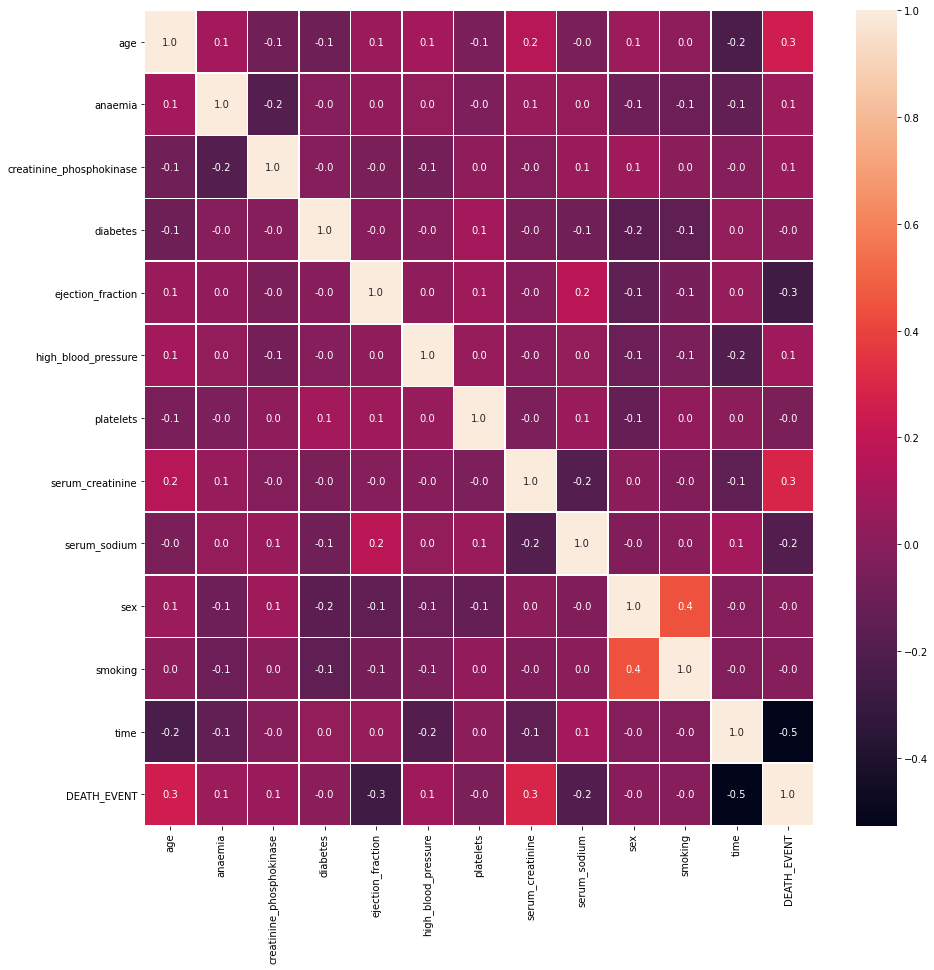
CORRELATION ANALYSIS TO UNDERSTAND THE INFLUENCE OF EACH FEATURE
f,ax = plt.subplots(figsize=(15, 15))
sns.heatmap(df.corr(), annot=True, linewidths=.5, fmt= '.1f',ax=ax)
plt.show()Clinical predictors of heart failure in patients with first acute myocardial infarction - "Predictors of early heart failure include previous medical conditions and age. The second peak occurrence can be predicted by similar characteristics in addition to increased peak creatine phosphokinase level, decreased left ventricular ejection fraction, and increased heart rate" (Am Heart J 1999;138:1133-9.)
Consideration :
Normal Values:
-
Creatine phosphokinase: 2 - 210 mcg/L
-
Ejection fraction : 50 %
-
Medical Follow-up : >=60 days
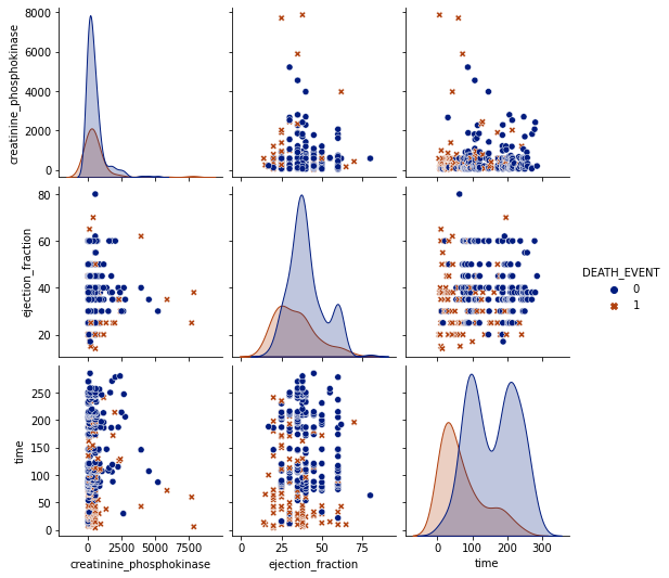
For this dataset, does creatine phosphokinase (increase) and ejection fraction (decrease) are behaving regarding a health valeu as the article metioned?
import seaborn as sns;
g1 = sns.pairplot(df,vars= ['creatinine_phosphokinase','ejection_fraction','time'], hue= 'DEATH_EVENT',markers=["o", "X" ],palette='dark')
% Death event of people who creatinine phosphokinase increased over normal, ejection fraction under normal and medical follow up under the stander 60 days :
H1 = df[['creatinine_phosphokinase', 'ejection_fraction','DEATH_EVENT','time']][(df['creatinine_phosphokinase'] > 210) & (df['ejection_fraction'] < 50) & (df['time'] < 60)]
H1['DEATH_EVENT'].mean()
0.92
% Death event of people who creatinine phosphokinase increased over normal, ejection fraction under normal and medical follow up under the stander 60 days :
H1 = df[['creatinine_phosphokinase', 'ejection_fraction','DEATH_EVENT','time']][(df['creatinine_phosphokinase'] > 210) & (df['ejection_fraction'] < 50) & (df['time'] >= 60)]
H1['DEATH_EVENT'].mean()
0.21367521367521367
Going a little deeper...
H1 = df[['creatinine_phosphokinase', 'ejection_fraction','DEATH_EVENT']][(df['creatinine_phosphokinase'] > 210) & (df['ejection_fraction'] < 50) & (df['DEATH_EVENT'] == 1)]
deathCr = H1['DEATH_EVENT'].count()
H1 = df[['creatinine_phosphokinase', 'ejection_fraction','DEATH_EVENT']][(df['creatinine_phosphokinase'] > 210) & (df['ejection_fraction'] < 50)]
print(r'%s pacients of 299 had values had not normal value for each feature. Representing %s percent of pacients and %s percent of total death. '%(H1.shape[0],round(((H1.shape[0]*100)/total),2), (deathCr*100)/total_death ))142 pacients of 299 had values had not normal value for each feature. Representing 47.49 percent of pacients and 50.0 percent of total death.
CONCLUSION
The value for creatinine phospkinase and ejection fraction are definitely significant for prediction of a heart failure. But a long-term medical follow-up must reduce drastically the chance of death. Which 92 % of the pacients passed away due heart failure who had creatinine phosphokinase's level above normal, ejection fraction under normal and medical follow-up less than 60 days. But, on another hand, only 21% with same creatinine and ejection fraction behavior and medical follow-up equal, or more, than 60 days passed away due a heart failure pacients
These unbalaced values are 47.5% of pacients and 50% of total of death in hole dataset.
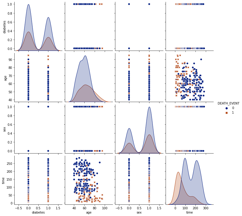
Role of Diabetes in Congestive Heart Failure - "Men aged 45 to 74 years had more than twice the frequency of congestive heart failure as their nondiabetic cohorts, and diabetic women had a fivefold increased risk."
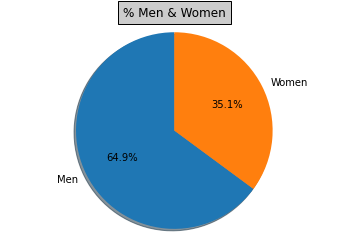
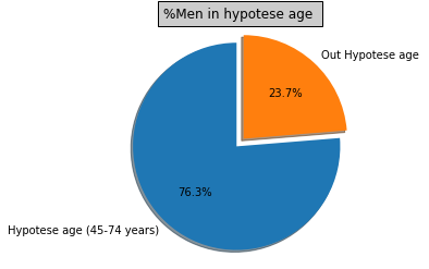
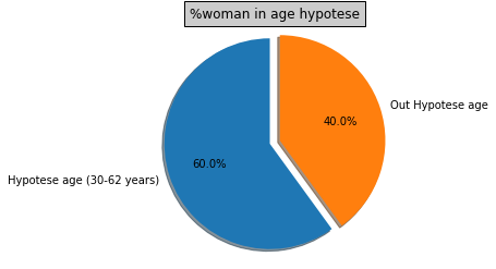
For this dataset, What the frequency of diabetic-men aged 45 to 74 years to had heart failure more than non-diabetic? What the same analyze for women 30 to 62 years ?
man   =  df['sex'][(df['sex'] == 1)]
woman =  df['sex'][(df['sex'] == 0)]

m = (man.count()*100)/total
w = (woman.count()*100)/total


import matplotlib.pyplot as plt

labels = 'Men','Women'
sizes  = [m,w]
explode = (0, 0)  # only "explode" the 2nd slice (i.e. 'Hogs')


fig1, ax1 = plt.subplots()
ax1.pie(sizes, explode=explode, labels=labels, autopct='%1.1f%%',
        shadow=True, startangle=90)
ax1.axis('equal')  # Equal aspect ratio ensures that pie is drawn as a circle.
plt.title("% Men & Women", bbox={'facecolor':'0.8', 'pad':5})
plt.show()

AM = df[['age','sex']][(df['sex'] == 1) & (df['age'] >= 45) & (df['age'] <= 74)]

labels = 'Hypotese age (45-74 years)','Out Hypotese age'
sizes  = [(AM.count()[0]*100)/man.count(),((man.count()-AM.count()[0])*100)/man.count()]
explode = (0.1, 0)  # only "explode" the 2nd slice (i.e. 'Hogs')


fig1, ax1 = plt.subplots()
ax1.pie(sizes, explode=explode, labels=labels, autopct='%1.1f%%',
        shadow=True, startangle=90)
ax1.axis('equal')  # Equal aspect ratio ensures that pie is drawn as a circle.
plt.title("%Men in hypotese age ", bbox={'facecolor':'0.8', 'pad':5})
plt.show()
g2 = sns.pairplot(df,vars= ['diabetes','age','sex','time'], hue= 'DEATH_EVENT',markers=["o", "X" ],palette='dark')N Death events to diabetic-men aged 45 to 74 years
H2 = df[['diabetes','age','sex','time','DEATH_EVENT']][(df['diabetes'] == 1) & (df['sex'] == 1) & (df['age'] >=45) & (df['age'] <= 74) & (df['DEATH_EVENT'] == 1)]
diab = H2['DEATH_EVENT'].count()
diab
16
N Death events to non-diabetic-men aged 45 to 74 years
H2 = df[['diabetes','age','sex','time','DEATH_EVENT']][(df['diabetes'] == 0) & (df['sex'] == 1) & (df['age'] >=45) & (df['age'] <= 74) & (df['DEATH_EVENT'] == 1)]
nodiab = H2['DEATH_EVENT'].count()
nodiab
26
Frequency (% Death events to diabetic-men) / (% Death events to non-diabetic-men)
diab/nodiab0.6153846153846154
AW = df[['age','sex']][(df['sex'] == 0) & (df['age'] >= 30) & (df['age'] <= 62)]

labels = 'Hypotese age (30-62 years)','Out Hypotese age'
sizes  = [(AW.count()[0]*100)/woman.count(),((woman.count()-AW.count()[0])*100)/woman.count()]
explode = (0, 0.1)  # only "explode" the 2nd slice (i.e. 'Hogs')

fig1, ax1 = plt.subplots()
ax1.pie(sizes, explode=explode, labels=labels, autopct='%1.1f%%',
        shadow=True, startangle=90)
ax1.axis('equal')  # Equal aspect ratio ensures that pie is drawn as a circle.
plt.title("%woman in age hypotese", bbox={'facecolor':'0.8', 'pad':5})
plt.show()
N Death events to diabetic-women aged 30 to 62 years
H2 = df[['diabetes','age','sex','time','DEATH_EVENT']][(df['diabetes'] == 1) & (df['sex'] == 0) & (df['age'] >=30) & (df['age'] <= 62) & (df['DEATH_EVENT'] == 1)]
diab = H2['DEATH_EVENT'].count()
diab
14
N Death events to non-diabetic-women aged 30 to 62 years
H2 = df[['diabetes','age','sex','time','DEATH_EVENT']][(df['diabetes'] == 0) & (df['sex'] == 0) & (df['age'] >=30) & (df['age'] <= 62) & (df['DEATH_EVENT'] == 1)]
nodiab = H2['DEATH_EVENT'].count()
nodiab
6
Frequency (% Death events to diabetic-women) / (% Death events to non-diabetic-women)
diab/nodiab2.3333333333333335
CONCLUSION
For this dataset, diabetic-men aged 45 to 74 years were less frequency (0.9 times) of death than non-diabetics Diabetic-women aged 30 to 62 year had more frequency (1.5 times) of death than non-diabetics.
The hypotese doens't correspond to the value expected although just Diabetic-women had a incresing on Death events but under de 5 times frequency.
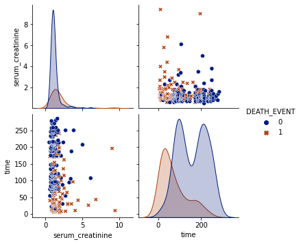
Effect of Elevated Admission Serum Creatinine and Its Worsening on Outcome in Hospitalized Patients With Decompensated Heart Failure - "Renal insufficiency (RI), as represented by elevated serum creatinine (>1.5 mg/dl) on admission, is common and found in almost half of patients hospitalized with decompensated heart failure"
Consideration :
Normal Values
serum creatinine: < 1.5 mg/dL
Medical Follow-up : <=60 days
For this dataset, what the correlation of serum creatinine and death events? Is the follow-up time is relevant?
g3 = sns.pairplot(df,vars= ['serum_creatinine','time'], hue= 'DEATH_EVENT',markers=["o", "X" ],palette='dark')H3 = df[['serum_creatinine','time','DEATH_EVENT']][(df['serum_creatinine'] > 1.5) & (df['time'] < 60) ]
deathCre = H3[(H3['DEATH_EVENT'] == 1)].count()
noDeathCre = H3[(H3['DEATH_EVENT'] == 0)].count()
total3 = H3.count()
#deathCre[0], noDeathCre[0],total3[0]Total number of patients with serum creatinine over normal value:
total3[0]23
Number of death event for total of patients with serum creatinine over normal value:
deathCre[0] 21
% Death Event in total
deathCre[0]*100/total3[0]91.30434782608695
%death events to follow-up over the 60 days:
H3 = df[['serum_creatinine','time','DEATH_EVENT']][(df['serum_creatinine'] > 1.5) & (df['time'] >= 60) ]
deathCre = H3[(H3['DEATH_EVENT'] == 1)].count()
noDeathCre = H3[(H3['DEATH_EVENT'] == 0)].count()

total3 = H3.count()
#deathCre[0], noDeathCre[0],total3[0]
deathCre[0]*100/total3[0]
50.0
Disregarding time, %Death events and total of pacients over >1.5 mg/dL
H3 = df[['serum_creatinine','DEATH_EVENT']][(df['serum_creatinine'] > 1.5)]
deathCre = H3[(H3['DEATH_EVENT'] == 1)].count()
noDeathCre = H3[(H3['DEATH_EVENT'] == 0)].count()

total3 = H3.count()
#deathCre[0], noDeathCre[0],total3[0]
deathCre[0]*100/total3[0], total3[0]
(64.17910447761194, 67)
CONCLUSION
The value for serum creatinine (SC) are definitely significant for prediction of a heart failure. Considering the follow-up time under of 60 days, the death events for pacients with SC over normal value is equal to 91.3 % (21 pacients) in the total of 23 pacients. For pacients who follow-up were over 60 days, the death event goes to 50% (22 pacients) of total of 44 pacients. From total of 67 pacients, 64% passed away.
Anaemia is an independent predictor of poor outcome in patients with chronic heart failure - "Mild anaemia is a significant and independent predictor of poor outcome in unselected patients with CHF."
What the relevance of anaemia to heart failure ?
H4 = df[['anaemia','DEATH_EVENT','time']]Number of pacients with anemia x without anemia
H4[(H4['anaemia']==1)].count()[0], H4[(H4['anaemia']==0)].count()[0](129, 170)
Number of pacients with anemia and passed away
H4[(H4['anaemia']==1) & (H4['DEATH_EVENT']==1)].count()[0]46
%Death anaemie pacient / total anaemie pacient
H4[(H4['anaemia']==1) & (H4['DEATH_EVENT']==1)].count()[0]*100/H4[(H4['anaemia']==1)].count()[0]35.65891472868217
H4[(H4['anaemia']==1) & (H4['time']<= 60)].count()[0], H4[(H4['anaemia']==0) & (H4['time']<= 60)].count()[0](33, 30)
H4[(H4['anaemia']==1) & (H4['DEATH_EVENT']==1) & (H4['time']<= 60)].count()[0]28
GENERAL OVERVIEW
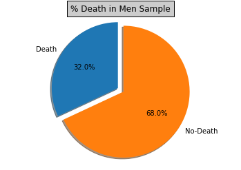
Death by gender
G1 = df[['sex','DEATH_EVENT']]m = G1[(G1['sex']==1) & (G1['DEATH_EVENT']==1)]
mdp = m['sex'].count()*100/G1[(G1['sex']==1)].count()[0]
w = G1[(G1['sex']==0) & (G1['DEATH_EVENT']==1)]
wdp = w['sex'].count()*100/G1[(G1['sex']==0)].count()[0]labels = 'Death','No-Death'
sizes = [mdp,100-mdp]
explode = (0.1, 0) # only "explode" the 2nd slice (i.e. 'Hogs')
fig1, ax1 = plt.subplots()
ax1.pie(sizes, explode=explode, labels=labels, autopct='%1.1f%%',
shadow=True, startangle=90)
ax1.axis('equal') # Equal aspect ratio ensures that pie is drawn as a circle.
plt.title("% Death in Men Sample", bbox={'facecolor':'0.8', 'pad':5})
plt.show()
labels = 'Death','No-Death'
sizes = [wdp,100-wdp]
explode = (0.1, 0) # only "explode" the 2nd slice (i.e. 'Hogs')
fig1, ax1 = plt.subplots()
ax1.pie(sizes, explode=explode, labels=labels, autopct='%1.1f%%',
shadow=True, startangle=90)
ax1.axis('equal') # Equal aspect ratio ensures that pie is drawn as a circle.
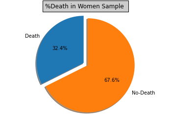
plt.title("%Death in Women Sample ", bbox={'facecolor':'0.8', 'pad':5})
plt.show()Death by Age
#### Death patient smokes x not
G3 = df[['smoking','DEATH_EVENT']]s = G3[(G3['smoking']==1) & (G3['DEATH_EVENT']==1)]
ns = G3[(G3['smoking']==0) & (G3['DEATH_EVENT']==1)]
Ts = G3[(G3['smoking']==1) & (G3['DEATH_EVENT']==0)]
Tns = G3[(G3['smoking']==0) & (G3['DEATH_EVENT']==0)]
#s.count()[0], Ts.count()[0], ns.count()[0], Tns.count()[0]labels = 'Death','No-Death'
sizes = [ns.count()[0]*100/(ns.count()[0]+Tns.count()[0]), Tns.count()[0]*100/(ns.count()[0]+Tns.count()[0])]
explode = (0.1, 0) # only "explode" the 2nd slice (i.e. 'Hogs')
fig1, ax1 = plt.subplots()
ax1.pie(sizes, explode=explode, labels=labels, autopct='%1.1f%%',
shadow=True, startangle=90)
ax1.axis('equal') # Equal aspect ratio ensures that pie is drawn as a circle.
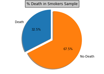
plt.title("% Death in Smokers Sample", bbox={'facecolor':'0.8', 'pad':5})
plt.show()
labels = 'Death','No-Death'
sizes = [wdp,100-wdp]
explode = (0.1, 0) # only "explode" the 2nd slice (i.e. 'Hogs')
fig1, ax1 = plt.subplots()
ax1.pie(sizes, explode=explode, labels=labels, autopct='%1.1f%%',
shadow=True, startangle=90)
ax1.axis('equal') # Equal aspect ratio ensures that pie is drawn as a circle.
plt.title("%Death in No-Smokers Sample ", bbox={'facecolor':'0.8', 'pad':5})
plt.show()Death patient with high blood pressure x not
Applying Machine Learning - Considering Time
import numpy as np%matplotlib inline
import seaborn as sns
import xgboost as xgb
from sklearn.model_selection import train_test_split
from sklearn.metrics import r2_score
from sklearn.preprocessing import LabelEncoder
from sklearn.preprocessing import StandardScaler
from sklearn.pipeline import make_pipeline
from sklearn.linear_model import LinearRegression
from sklearn.model_selection import GridSearchCV
from sklearn.svm import LinearSVR , SVR
from sklearn.tree import DecisionTreeRegressor
from sklearn.ensemble import RandomForestRegressor
from xgboost import XGBRegressor
from sklearn.model_selection import train_test_split , KFold , cross_val_score,StratifiedKFold
from sklearn.metrics import mean_absolute_error , mean_squared_error
from sklearn.preprocessing import OneHotEncoder
from sklearn.feature_selection import SelectFromModel
from sklearn.linear_model import ElasticNet, Lasso, Ridge
from sklearn.feature_selection import SelectKBest
from sklearn.feature_selection import f_classif
from xgboost import XGBClassifier
from sklearn.datasets import load_iris
from sklearn.metrics import confusion_matrix
from sklearn.model_selection import train_test_split
from sklearn.model_selection import cross_val_score, KFold
from sklearn.ensemble import RandomForestClassifier
from sklearn.tree import DecisionTreeClassifier
from sklearn.ensemble import RandomForestClassifier
from sklearn.datasets import make_classification
import functools
import sys
import warnings
if not sys.warnoptions:
warnings.simplefilter("ignore")X = df.drop('DEATH_EVENT',axis=1)
y = df['DEATH_EVENT']
X_train,X_test,y_train,y_test = train_test_split(X,y,test_size = 0.3,random_state = 42)def cross_valid (model,name,X = X_train , y= y_train):
modelo = model()
cv = 5 #quantidade de vezes q vai rodar
scoring = 'neg_mean_squared_error' # funcão mse dentro do cross_validation_score
n_jobs = -1
score = cross_val_score(modelo,X ,y , cv= cv , scoring= scoring, n_jobs= n_jobs)
RMSE = np.sqrt(- score.mean())
##menor melhor
print('RMSE',name,RMSE)cross_valid(RandomForestRegressor,'random_forest')RMSE random_forest 0.3310877086934085
cross_valid(XGBRegressor,'xg_boost')RMSE xg_boost 0.3555536909123532
cross_valid(Lasso,'lasso')RMSE lasso 0.3838246741795928
cross_valid(Ridge,'ridge')RMSE ridge 0.3536173277735311
cross_valid(SVR,'SVR')RMSE SVR 0.48558580486692
cross_valid(LinearSVR,'Linear_SVR')RMSE Linear_SVR 0.6336108098091258
cross_valid(XGBClassifier,'XGBClassifier')RMSE XGBClassifier 0.3849672294000657
cross_valid(DecisionTreeClassifier,'Decision_tree')RMSE Decision_tree 0.42044166811032346
cross_valid(RandomForestClassifier,'RandomForestClassifier')RMSE RandomForestClassifier 0.3656251706175088
X = df.drop('DEATH_EVENT',axis=1)
y = df['DEATH_EVENT']plt.figure(figsize=(13,6))
dt=RandomForestClassifier()
dt.fit(X,y)
feat_importances1 = pd.Series(dt.feature_importances_, index=X.columns)
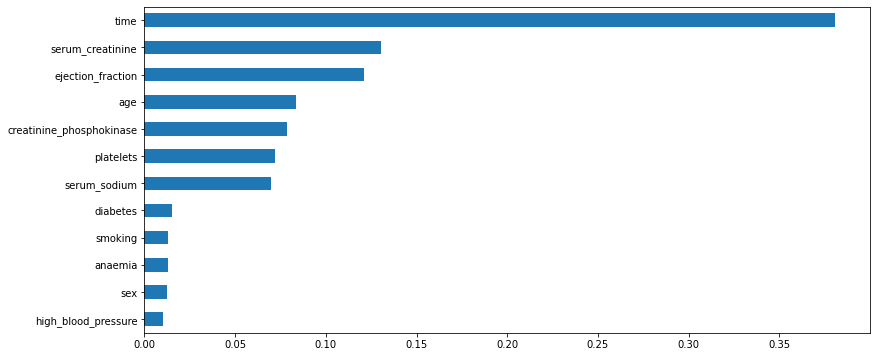
feat_importances1.sort_values(ascending=True).plot(kind='barh')
plt.show()feat_importances1.head(14)age 0.083395
anaemia 0.013054
creatinine_phosphokinase 0.078637
diabetes 0.015090
ejection_fraction 0.120798
high_blood_pressure 0.010296
platelets 0.071771
serum_creatinine 0.130493
serum_sodium 0.069820
sex 0.012747
smoking 0.013187
time 0.380713
dtype: float64
param_grid = {
            "n_estimators"      : [10,50,100,200,700],
            "max_features"      : ["auto", "sqrt", "log2"],
            "min_samples_split" : [2,4,8],
            "bootstrap": [True, False],
            }
grid =GridSearchCV(RandomForestClassifier(), param_grid, cv=5,
n_jobs=-1, verbose=1)
grid.fit(X_train, y_train)Fitting 5 folds for each of 90 candidates, totalling 450 fits
[Parallel(n_jobs=-1)]: Using backend LokyBackend with 2 concurrent workers.
[Parallel(n_jobs=-1)]: Done 60 tasks | elapsed: 13.1s
[Parallel(n_jobs=-1)]: Done 210 tasks | elapsed: 51.3s
[Parallel(n_jobs=-1)]: Done 450 out of 450 | elapsed: 1.7min finished
GridSearchCV(cv=5, error_score=nan,
estimator=RandomForestClassifier(bootstrap=True, ccp_alpha=0.0,
class_weight=None,
criterion='gini', max_depth=None,
max_features='auto',
max_leaf_nodes=None,
max_samples=None,
min_impurity_decrease=0.0,
min_impurity_split=None,
min_samples_leaf=1,
min_samples_split=2,
min_weight_fraction_leaf=0.0,
n_estimators=100, n_jobs=None,
oob_score=False,
random_state=None, verbose=0,
warm_start=False),
iid='deprecated', n_jobs=-1,
param_grid={'bootstrap': [True, False],
'max_features': ['auto', 'sqrt', 'log2'],
'min_samples_split': [2, 4, 8],
'n_estimators': [10, 50, 100, 200, 700]},
pre_dispatch='2*n_jobs', refit=True, return_train_score=False,
scoring=None, verbose=1)
RMSE_grid_param = np.sqrt(grid.best_score_)

RMSE_grid_param
0.9384050025956979
grid.best_params_{'bootstrap': True,
'max_features': 'auto',
'min_samples_split': 4,
'n_estimators': 100}
pred = grid.predict(X_test)
pred
array([0, 0, 0, 1, 0, 0, 0, 0, 1, 0, 0, 0, 0, 0, 1, 1, 0, 0, 0, 0, 0, 0,
1, 1, 1, 0, 0, 0, 0, 0, 1, 0, 1, 1, 1, 1, 0, 0, 0, 0, 0, 1, 0, 0,
0, 0, 0, 0, 0, 0, 0, 0, 0, 0, 0, 0, 0, 1, 0, 1, 1, 1, 0, 0, 1, 1,
0, 1, 0, 0, 1, 0, 0, 0, 0, 0, 0, 1, 0, 0, 0, 1, 0, 0, 0, 0, 0, 1,
1, 0])
score = r2_score(y_test,pred)
score
0.08210096889342178
MSE = mean_squared_error(y_test,pred)
MSE
0.2222222222222222
RMSE_pred = np.sqrt(MSE)
RMSE_pred
0.4714045207910317
pred2 = grid.predict(X_train)
MSE2 = mean_squared_error(y_train,pred2)
RMSE2_pred = np.sqrt(MSE2)
RMSE2_pred
0.0
import pandas as pd
import seaborn as sn
import matplotlib.pyplot as plt

data = {'y_Actual':    y_test,
        'y_Predicted': pred
        }

dft = pd.DataFrame(data, columns=['y_Actual','y_Predicted'])
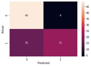
confusion_matrix = pd.crosstab(dft['y_Actual'], dft['y_Predicted'], rownames=['Actual'], colnames=['Predicted'])

sn.heatmap(confusion_matrix, annot=True)
plt.show()
Applying Machine Learning - Without Time
X = df.drop(['DEATH_EVENT', 'time'],axis=1)
y = df['DEATH_EVENT']
X_train,X_test,y_train,y_test = train_test_split(X,y,test_size = 0.3,random_state = 42)
def cross_valid (model,name,X = X_train , y= y_train):
modelo = model()
cv = 5 #quantidade de vezes q vai rodar
scoring = 'neg_mean_squared_error' # funcão mse dentro do cross_validation_score
n_jobs = -1
score = cross_val_score(modelo,X ,y , cv= cv , scoring= scoring, n_jobs= n_jobs)
RMSE = np.sqrt(- score.mean())
##menor melhor
print('RMSE',name,RMSE)cross_valid(RandomForestClassifier,'RandomForestClassifier')RMSE RandomForestClassifier 0.4637873676759594
cross_valid(RandomForestRegressor,'random_forest')RMSE random_forest 0.3977204207745
cross_valid(XGBRegressor,'xg_boost')RMSE xg_boost 0.40968810731337457
cross_valid(Lasso,'lasso')RMSE lasso 0.4512461871781548
cross_valid(Ridge,'ridge')RMSE ridge 0.41835811411245727
cross_valid(SVR,'SVR')RMSE SVR 0.4855765692487356
cross_valid(LinearSVR,'Linear_SVR')RMSE Linear_SVR 0.9000051885995444
cross_valid(XGBClassifier,'XGBClassifier')RMSE XGBClassifier 0.4985460859015062
cross_valid(DecisionTreeClassifier,'Decision_tree')RMSE Decision_tree 0.5312532024908597
cross_valid(RandomForestClassifier,'RandomForestClassifier')RMSE RandomForestClassifier 0.45887809458619494
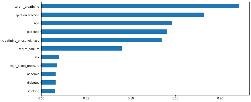
plt.figure(figsize=(13,6))
dt=RandomForestRegressor()
dt.fit(X,y)
feat_importances1 = pd.Series(dt.feature_importances_, index=X.columns)
feat_importances1.sort_values(ascending=True).plot(kind='barh')
plt.show()X_train,X_test,y_train,y_test = train_test_split(X,y,test_size = 0.3,random_state = 42)param_grid = {
"n_estimators" : [10,50,100,200],
"max_features" : ["auto", "sqrt", "log2"],
"min_samples_split" : [2,4,8],
"bootstrap": [True, False],
}grid =GridSearchCV(RandomForestClassifier(), param_grid, cv=5,
n_jobs=-1, verbose=1)
grid.fit(X_train, y_train)Fitting 5 folds for each of 72 candidates, totalling 360 fits
[Parallel(n_jobs=-1)]: Using backend LokyBackend with 2 concurrent workers.
[Parallel(n_jobs=-1)]: Done 164 tasks | elapsed: 17.9s
[Parallel(n_jobs=-1)]: Done 360 out of 360 | elapsed: 36.0s finished
GridSearchCV(cv=5, error_score=nan,
estimator=RandomForestClassifier(bootstrap=True, ccp_alpha=0.0,
class_weight=None,
criterion='gini', max_depth=None,
max_features='auto',
max_leaf_nodes=None,
max_samples=None,
min_impurity_decrease=0.0,
min_impurity_split=None,
min_samples_leaf=1,
min_samples_split=2,
min_weight_fraction_leaf=0.0,
n_estimators=100, n_jobs=None,
oob_score=False,
random_state=None, verbose=0,
warm_start=False),
iid='deprecated', n_jobs=-1,
param_grid={'bootstrap': [True, False],
'max_features': ['auto', 'sqrt', 'log2'],
'min_samples_split': [2, 4, 8],
'n_estimators': [10, 50, 100, 200]},
pre_dispatch='2*n_jobs', refit=True, return_train_score=False,
scoring=None, verbose=1)
RMSE_grid_param = np.sqrt(grid.best_score_)
RMSE_grid_param
0.8939725901110832
grid.best_params_{'bootstrap': True,
'max_features': 'log2',
'min_samples_split': 4,
'n_estimators': 200}
pred = grid.predict(X_test)
pred
array([1, 0, 0, 1, 0, 0, 0, 0, 1, 1, 0, 0, 0, 0, 0, 0, 0, 0, 0, 0, 0, 0,
1, 0, 0, 0, 0, 0, 0, 0, 1, 0, 0, 1, 0, 0, 0, 1, 0, 0, 0, 1, 0, 0,
1, 0, 1, 0, 0, 0, 0, 0, 0, 0, 0, 0, 0, 1, 0, 1, 1, 1, 0, 0, 1, 0,
0, 1, 0, 0, 1, 1, 0, 0, 1, 0, 0, 0, 0, 0, 0, 1, 0, 0, 0, 0, 0, 0,
1, 0])
score = r2_score(y_test,pred)
score
-0.4227434982151961
MSE = mean_squared_error(y_test,pred)
MSE
0.34444444444444444
RMSE_pred = np.sqrt(MSE)
RMSE_pred
0.5868938953886337
import pandas as pd
import seaborn as sn
import matplotlib.pyplot as plt

data = {'y_Actual':    y_test,
        'y_Predicted': pred
        }

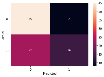
dft = pd.DataFrame(data, columns=['y_Actual','y_Predicted'])
confusion_matrix = pd.crosstab(dft['y_Actual'], dft['y_Predicted'], rownames=['Actual'], colnames=['Predicted'])

sn.heatmap(confusion_matrix, annot=True)
plt.show()