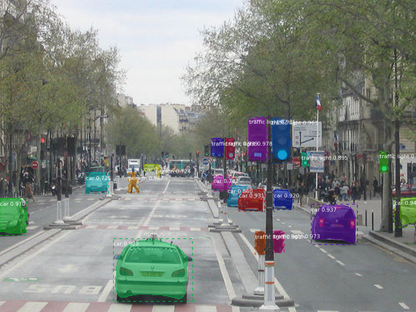
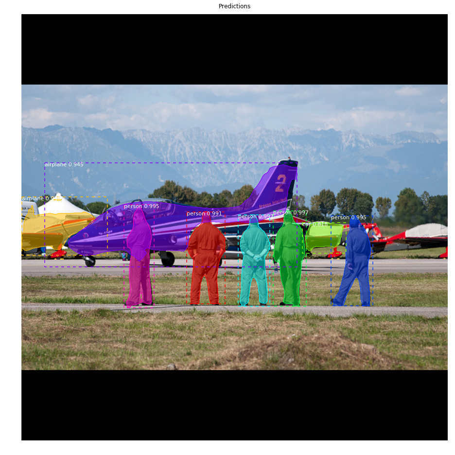
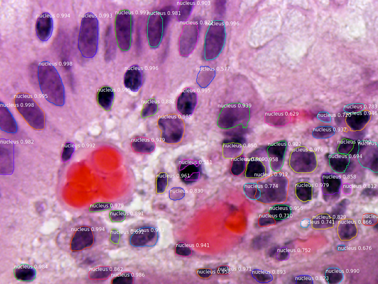
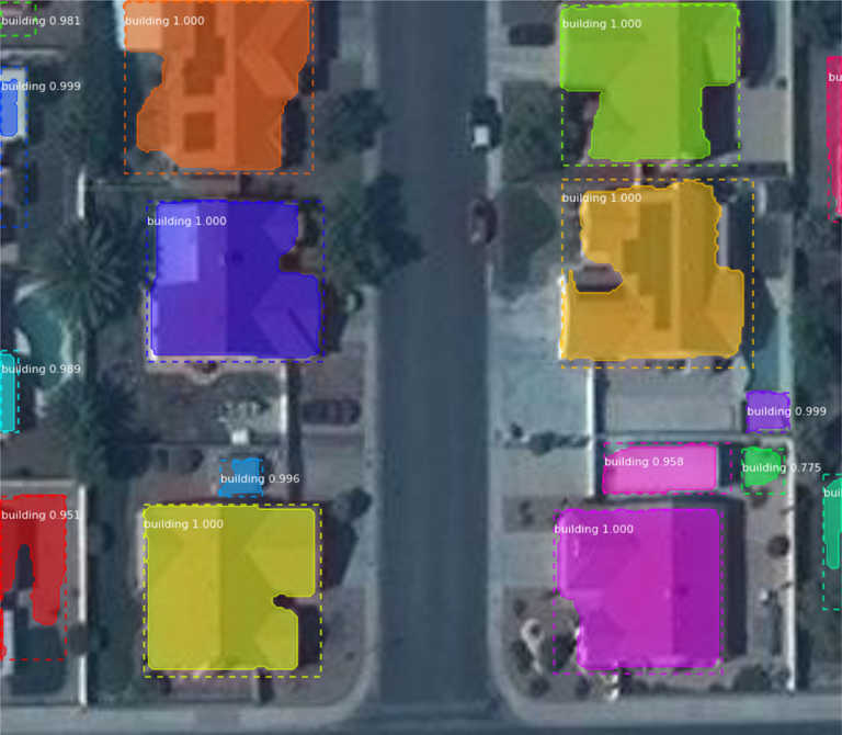
This solution is based on Matterport's Mask_RCNN implementation on keras/tensorflow. Please look at the original repository (https://github.com/matterport/Mask_RCNN) for specific details. This is an implementation of Mask R-CNN on Python 3, Keras, and TensorFlow. The model generates bounding boxes and segmentation masks for each instance of an object in the image. It's based on Feature Pyramid Network (FPN) and a ResNet101 backbone. I have used the pretrained COCO weights as the starting point for my training on the nuclei segmentation dataset.
Some of the Mask-RCNN files are modified, in particular model.py and utils.py.
I did not use any additional external data. Training was done with a modified version of the dataset as in the discussion forum: https://www.kaggle.com/c/data-science-bowl-2018/discussion/50518 and mentioned several times in the Official External Data thread as a link to: https://github.com/lopuhin/kaggle-dsbowl-2018-dataset-fixes For stage2 I didn't retrain my model with the released stage1_test images. File my_bowl_dataset.py generates the bowldataset class to upload the images and masks in the correct format.
The modifications of files model.py and utils.py are needed for scaling the training set images before random 512x512 crops are taken for training. This scaling that take places in the "resize_image" function in utils.py and also includes aspect ratio changes of the images. In addition, code in model.py inside the "augment" section of function "load_image_gt", allows for further image augmentation of the 512x512 crops, concretely:
- vertical and horizontal flips
- 90 degree rotations
- further rotation by random angles.
- color channel shift (this function is copied from the keras Imagegenerator function).
Similar augmentations can be achieved with the imgaug library (see the code for an example), but I have found these slightly underperform compared to my implementation. Also note that my winning implementation contained a bug that I have removed from this source code, so the results of running the training schedule bellow vary slightly from my final implementation. The bug was in the cropping function in utils.py and resulted in my code always taking the same part of an image (after the random rescaling that was working ok). Surprisingly, this bug did not penalize much my score, although I would have gone up one or maybe two positions if I hadn't made this stupid error.....
Training takes place in three consecutive steps.
For the first step we initialized the network with the COCO weights pretrained by Matterport (mentioned in the External data thread) and accessible at: https://github.com/matterport/Mask_RCNN/releases/download/v2.0/mask_rcnn_coco.h5 File "my_train_1.py" contains the code for the first training step. This is the most important part of the training, the other two steps don't improve much. Training doesn't have anything fancy, it just trains for 75 epochs, reducing the learning rate at epoch 30 and 50. Training uses the default SGD.
File "my_train_2.py" contains the second step. In this step we initialize the network with the final epoch weights in step 1. We then train for 40 additional epochs. The difference with step 1 is how images are taken from the training set. In step 1 images are taken one at a time as in most training procedures. But it is easy to see that the types of images and the number of each type are quite different, this makes the training dataset quite unbalanced in regards to the type of images to classify. Because the training set had groups of images of different sizes and usually the smaller images are more abundant I thought that it would be good (given all the cropping done above) that for each epoch we use several times the same image, in particular for the larger images. In summary , the train set as provided has 9 image sizes, each with different number of images: (256, 320, 4) 111 (1040, 1388, 4) 1 (360, 360, 4) 90 (260, 347, 4) 3 (512, 640, 4) 13 (603, 1272, 4) 6 (256, 256, 4) 334 (1024, 1024, 4) 16 (520, 696, 4) 90 So I take 334 copies of the (1040,1388) image and add them to the training set, I take 1 copy of each image in the (256,256) category, 3 copies of each image in the (256,320) category and so on generating a training set that has the same number of images of each size. This makes my training set very large...
File "my_train_3.py" contains the third step. The final third step takes the weights of the last epoch in Step 2 and repeats the same procedure for a further 5 epochs with slightly larger augmentation parameters. The resulting weights are what have been used for my winning solution. It should be noted, however, that Steps 2 and 3 do not result in significant improvement of the Step 2 predictions (it is easy to say now that we can see the scores... ;) ). The weights for my solution are too large for github, you can download them at : https://drive.google.com/file/d/19kVton20JL9u0CpwGssD7EbBvsWcq1ty/view?usp=sharing
Inference uses the "pad64" option of Matterport's Mask_RCNN implementation.
-
my_inference.py contains a basic inference for the test set. Adding a binary dilation operation as simple postprocessing. This is a simplified version that results in equally good results as the test time augmentation (tta) used in my final solution. In fact, I would recommend using this version, the tta has a lot of parameters to tweak and (again it is easy to say when you can see the stage 2 results...) in my opinion it is not really worth it.
-
my_inference_tta.py For each image we make 15 predictions using the same model but different test time augmentations. This takes a long time for the 3k images in the final stage2, in fact, my final solution did not use the multiproccessing that I have added later and speeds up things quite a lot. The 15 augmentations used are based on different combinations of flips 90 degree rotations, channel shift ranges and scaling of the width and length. These are specified in the aug_options list. For example an entry [True, False, 2,7,1.1,1.2] will make an upside-down flip, no left-right flip, rotate 90 degrees two times, randomly shift the channels with a value of 7 and scale the image with a width scaling of 1.1 and height scaling of 1.2. Once the 15 predictions for each image are performed we merge the predictions. The function that merges the test time augmentations (TTA) is quite complex so I've tried to document what is going on as much as possible in that python file. As I said, a binary dilation operation on a single prediction (this is not part of my winning solution but I include it in the code) achieves similar results and takes much less time. Also note that this tta hyperparameters are set for my solution that includes the bug documented above. If you want to reproduce the exact result you should include the bug in the image "random" cropping. This code generates the csv file with the run-length encoding that were submitted as the 3th place solution.
This is an implementation of Mask R-CNN on Python 3, Keras, and TensorFlow. The model generates bounding boxes and segmentation masks for each instance of an object in the image. It's based on Feature Pyramid Network (FPN) and a ResNet101 backbone.
The repository includes:
- Source code of Mask R-CNN built on FPN and ResNet101.
- Training code for MS COCO
- Pre-trained weights for MS COCO
- Jupyter notebooks to visualize the detection pipeline at every step
- ParallelModel class for multi-GPU training
- Evaluation on MS COCO metrics (AP)
- Example of training on your own dataset
The code is documented and designed to be easy to extend. If you use it in your research, please consider referencing this repository. If you work on 3D vision, you might find our recently released Matterport3D dataset useful as well. This dataset was created from 3D-reconstructed spaces captured by our customers who agreed to make them publicly available for academic use. You can see more examples here.
-
demo.ipynb Is the easiest way to start. It shows an example of using a model pre-trained on MS COCO to segment objects in your own images. It includes code to run object detection and instance segmentation on arbitrary images.
-
train_shapes.ipynb shows how to train Mask R-CNN on your own dataset. This notebook introduces a toy dataset (Shapes) to demonstrate training on a new dataset.
-
(model.py, utils.py, config.py): These files contain the main Mask RCNN implementation.
-
inspect_data.ipynb. This notebook visualizes the different pre-processing steps to prepare the training data.
-
inspect_model.ipynb This notebook goes in depth into the steps performed to detect and segment objects. It provides visualizations of every step of the pipeline.
-
inspect_weights.ipynb This notebooks inspects the weights of a trained model and looks for anomalies and odd patterns.
To help with debugging and understanding the model, there are 3 notebooks (inspect_data.ipynb, inspect_model.ipynb, inspect_weights.ipynb) that provide a lot of visualizations and allow running the model step by step to inspect the output at each point. Here are a few examples:
Visualizes every step of the first stage Region Proposal Network and displays positive and negative anchors along with anchor box refinement.

This is an example of final detection boxes (dotted lines) and the refinement applied to them (solid lines) in the second stage.
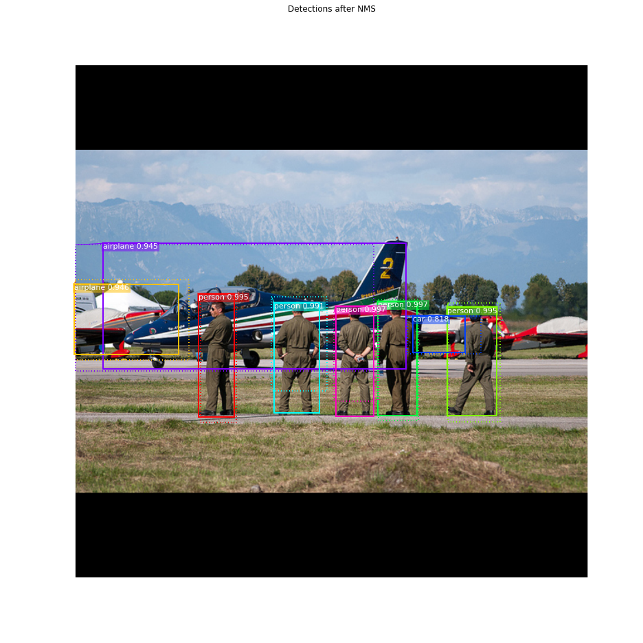
Examples of generated masks. These then get scaled and placed on the image in the right location.
Often it's useful to inspect the activations at different layers to look for signs of trouble (all zeros or random noise).
Another useful debugging tool is to inspect the weight histograms. These are included in the inspect_weights.ipynb notebook.
TensorBoard is another great debugging and visualization tool. The model is configured to log losses and save weights at the end of every epoch.
We're providing pre-trained weights for MS COCO to make it easier to start. You can
use those weights as a starting point to train your own variation on the network.
Training and evaluation code is in samples/coco/coco.py. You can import this
module in Jupyter notebook (see the provided notebooks for examples) or you
can run it directly from the command line as such:
# Train a new model starting from pre-trained COCO weights
python3 samples/coco/coco.py train --dataset=/path/to/coco/ --model=coco

# Train a new model starting from ImageNet weights
python3 samples/coco/coco.py train --dataset=/path/to/coco/ --model=imagenet

# Continue training a model that you had trained earlier
python3 samples/coco/coco.py train --dataset=/path/to/coco/ --model=/path/to/weights.h5

# Continue training the last model you trained. This will find
# the last trained weights in the model directory.
python3 samples/coco/coco.py train --dataset=/path/to/coco/ --model=last
You can also run the COCO evaluation code with:
# Run COCO evaluation on the last trained model
python3 samples/coco/coco.py evaluate --dataset=/path/to/coco/ --model=last
The training schedule, learning rate, and other parameters should be set in samples/coco/coco.py.
Start by reading this blog post about the balloon color splash sample. It covers the process starting from annotating images to training to using the results in a sample application.
In summary, to train the model on your own dataset you'll need to extend two classes:
Config
This class contains the default configuration. Subclass it and modify the attributes you need to change.
Dataset
This class provides a consistent way to work with any dataset.
It allows you to use new datasets for training without having to change
the code of the model. It also supports loading multiple datasets at the
same time, which is useful if the objects you want to detect are not
all available in one dataset.
See examples in samples/shapes/train_shapes.ipynb, samples/coco/coco.py, samples/balloon/balloon.py, and samples/nucleus/nucleus.py.
This implementation follows the Mask RCNN paper for the most part, but there are a few cases where we deviated in favor of code simplicity and generalization. These are some of the differences we're aware of. If you encounter other differences, please do let us know.
-
Image Resizing: To support training multiple images per batch we resize all images to the same size. For example, 1024x1024px on MS COCO. We preserve the aspect ratio, so if an image is not square we pad it with zeros. In the paper the resizing is done such that the smallest side is 800px and the largest is trimmed at 1000px.
-
Bounding Boxes: Some datasets provide bounding boxes and some provide masks only. To support training on multiple datasets we opted to ignore the bounding boxes that come with the dataset and generate them on the fly instead. We pick the smallest box that encapsulates all the pixels of the mask as the bounding box. This simplifies the implementation and also makes it easy to apply image augmentations that would otherwise be harder to apply to bounding boxes, such as image rotation.
To validate this approach, we compared our computed bounding boxes to those provided by the COCO dataset. We found that ~2% of bounding boxes differed by 1px or more, ~0.05% differed by 5px or more, and only 0.01% differed by 10px or more.
-
Learning Rate: The paper uses a learning rate of 0.02, but we found that to be too high, and often causes the weights to explode, especially when using a small batch size. It might be related to differences between how Caffe and TensorFlow compute gradients (sum vs mean across batches and GPUs). Or, maybe the official model uses gradient clipping to avoid this issue. We do use gradient clipping, but don't set it too aggressively. We found that smaller learning rates converge faster anyway so we go with that.
Contributions to this repository are welcome. Examples of things you can contribute:
- Speed Improvements. Like re-writing some Python code in TensorFlow or Cython.
- Training on other datasets.
- Accuracy Improvements.
- Visualizations and examples.
You can also join our team and help us build even more projects like this one.
Python 3.4, TensorFlow 1.3, Keras 2.0.8 and other common packages listed in requirements.txt.
To train or test on MS COCO, you'll also need:
- pycocotools (installation instructions below)
- MS COCO Dataset
- Download the 5K minival and the 35K validation-minus-minival subsets. More details in the original Faster R-CNN implementation.
If you use Docker, the code has been verified to work on this Docker container.
-
Install dependencies
pip3 install -r requirements.txt
-
Clone this repository
-
Run setup from the repository root directory
python3 setup.py install
-
Download pre-trained COCO weights (mask_rcnn_coco.h5) from the releases page.
-
(Optional) To train or test on MS COCO install
pycocotoolsfrom one of these repos. They are forks of the original pycocotools with fixes for Python3 and Windows (the official repo doesn't seem to be active anymore).- Linux: https://github.com/waleedka/coco
- Windows: https://github.com/philferriere/cocoapi. You must have the Visual C++ 2015 build tools on your path (see the repo for additional details)
If you extend this model to other datasets or build projects that use it, we'd love to hear from you.
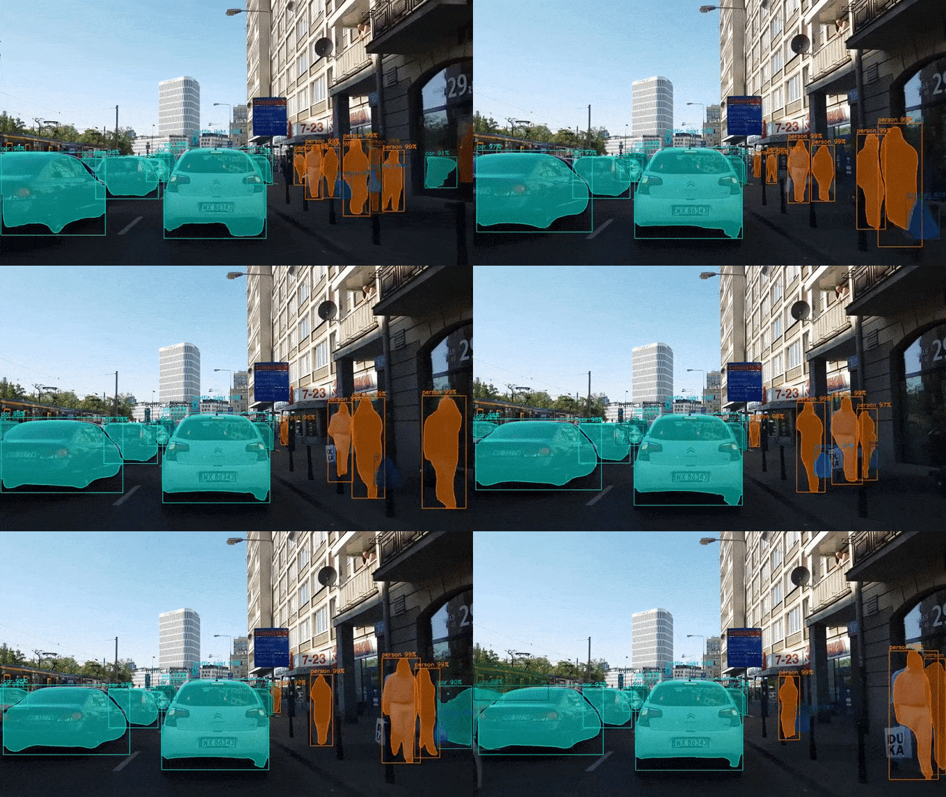
4K Video Demo by Karol Majek.
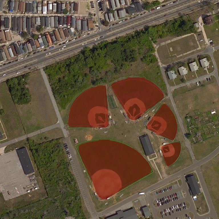
Images to OSM: Improve OpenStreetMap by adding baseball, soccer, tennis, football, and basketball fields.
Splash of Color. A blog post explaining how to train this model from scratch and use it to implement a color splash effect.
Segmenting Nuclei in Microscopy Images. Built for the 2018 Data Science Bowl
Code is in the samples/nucleus directory.
