python-ml-snippets: A repository from Lucasus

What can you find here?

Useful Python code snippets, helpful when working on machine learning modesl with scikit-learn and pandas

Snippets are below:

Create Conda environment

Run following command in Anaconda Prompt (Windows) to create Conda environment. We also install optionally tensorflow

conda create -n coder python=3.6 anaconda
conda install -n coder -c conda-forge tensorflow

Running notebook

Running Jupyter notebook:

jupyter notebook

Running Jupyter lab:

jupyter lab

Notebook configuration (magic functions)

#To display inline plots:
%matplotlib inline

#To get autocompletion:
%config IPCompleter.greedy=True

Loading data

import pandas as pd

# Load data from csv file, file doesn't have header column
# plus setting type of some column 
df = pd.read_csv(
    "dataset.csv", 
    header = None, 
    sep = ';',
    names = ['column_name1', 'column_name2'],
    dtype={'column_name2':np.int})
    
# Load data from csv, comma as decimal separator, header row exists    
df = pd.read_csv("dataset.csv", sep = ';', decimal=",")

Getting basic info about data

# df is pandas dataframe

# Get first 5 rows
df.head() 

# Get information about data types, number of rows
df.info()

# Get basic distribution information
df.describe()

# Get basic distribution information including categorical columns
df.describe(include='all')

Data analysis

Get distribution of categorical column values:

pp(df['some_column'].value_counts())

Data manipulation

Very useful snippets: https://gist.github.com/bsweger/e5817488d161f37dcbd2

Transforming single column

df['positive_amount'] = df['amount'].apply(lambda x: x > 0)

Simple filtering

# Returns df rows with amount < 0
df[(df['amount']<0)]

Training / test sets preparation

Taking first 80% of rows as training set, remaining as test set

from sklearn.model_selection import train_test_split
X = df.loc[:,["attribute_1", "attribute_2", "attribute_3", "attribute_4"]]
y = df.loc[:, "label"]
X_train, X_test, y_train, y_test = train_test_split(X, y, test_size = 0.20, shuffle = False)

Taking 80% of random rows as training set, remaining as test set

from sklearn.model_selection import train_test_split
X = df.loc[:,["attribute_1", "attribute_2", "attribute_3", "attribute_4"]]
y = df.loc[:, "label"]
X_train, X_test, y_train, y_test = train_test_split(X, y, test_size = 0.20, random_state=42)

Plotting

Configuration

#Configure default size of plots in Jupyter Notebook (mostly to make them bigger)
import matplotlib.pyplot as plt
plt.rcParams['figure.figsize'] = [16, 8]

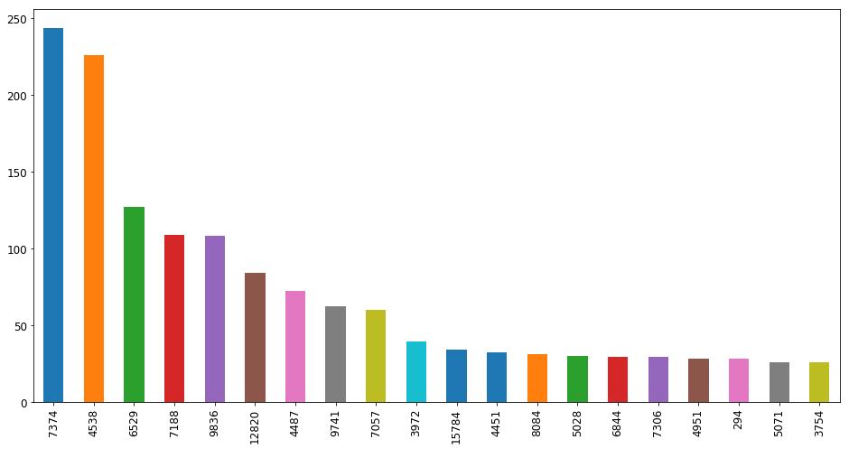
Plot distibution of some value - sort by occurence count, show top 20

import pandas as pd
pd.value_counts(df['some_column']).nlargest(20).plot.bar()

Result:

Displaying scatter matrix (to look for correlations)

from pandas.plotting import scatter_matrix
attributes = ["column_1", "column_2", "column_n"]
scatter_matrix(df[attributes], figsize=(12,8))

Displaying scatter plot to check in detail correlation between two attributes

df.plot(kind="scatter", x = "column_1", y = "column_2", alpha = 0.1)

Lucasus/python-ml-snippets