sgpvalue

The goal of sgpvalue is to help bring clarity to the Second Generation P-value paper.

Installation

# install.packages("devtools")
devtools::install_github("LucyMcGowan/sgpvalue")

Example

The p_delta() function will calculate the Second Generation P-value give the 95% interval (lb, ub) and indifference zone (delta_lb, delta_ub).

library(sgpvalue)
p_delta(lb = 145, ub = 148, delta_lb = 147, delta_ub = 149)
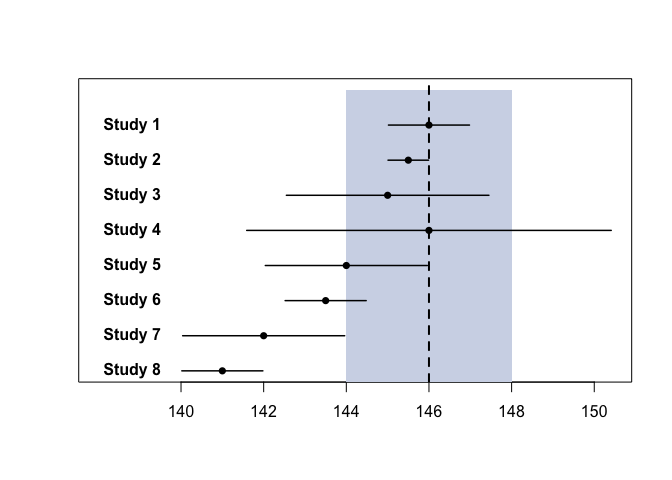
#> [1] 0.3333333

Comparison to traditional methods

The compare_p() function allows the user to compare Traditional Maximum p-values, and Second Generation P-values for given studies. For example, below are mock results from 8 studies of systolic blood pressure. Here the point null is 146 mmHg, indicated by the vertical dashed line, with an indifference zone, or interval null hypothesis, from 144 mmHg to 148 mmHg shaded in blue-grey (Figure 2 from the Second Generation P-value paper).

data <- data.frame(
   xbar = c(146, 145.5, 145, 146, 144, 143.5, 142, 141),
   se = c(0.5, 0.25, 1.25, 2.25, 1, 0.5, 1, 0.5)
   )
compare_p(data, delta_lb = 144, delta_ub = 148, h0 = 146)

#>    xbar   se     lb     ub   p_old   p_max     p_new
#> 1 146.0 0.50 145.02 146.98 1.00000 1.00000 1.0000000
#> 2 145.5 0.25 145.01 145.99 0.04550 1.00000 1.0000000
#> 3 145.0 1.25 142.55 147.45 0.42371 1.00000 0.7040816
#> 4 146.0 2.25 141.59 150.41 1.00000 1.00000 0.5000000
#> 5 144.0 1.00 142.04 145.96 0.04550 1.00000 0.5000000
#> 6 143.5 0.50 142.52 144.48 0.00000 0.31731 0.2448980
#> 7 142.0 1.00 140.04 143.96 0.00006 0.04550 0.0000000
#> 8 141.0 0.50 140.02 141.98 0.00000 0.00000 0.0000000

Operating characteristics

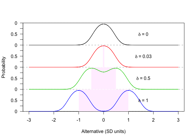
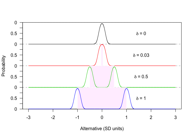
You can observe the operating characteristics using the power_curves() function. This allows you to input n and varying delta values and observe power curves for the null, alternative, or inconclusive p_delta values.

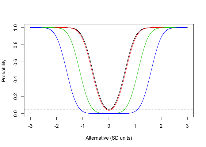
Figure S3 from the second generation P-value paper. The relationship between the probability that p_delta = 0 varying delta.

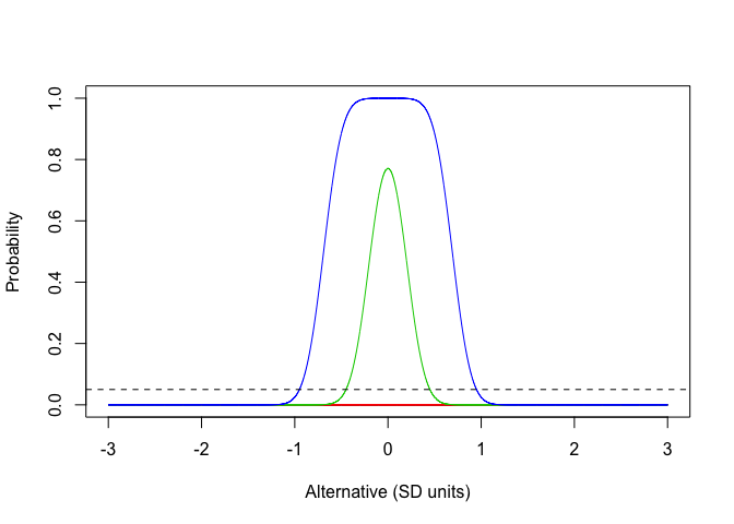
power_curves(delta = c(0, 1/30, 1/2, 1), n = 10, prob = "null")

Figure S5 from the second generation P-value paper. The relationship between probability of data supported compatibility 517 with the null hypothesis, and various deltas.

## n = 40 (Figure S5 left)
power_curves(delta = c(0, 1/30, 1/2, 1), n = 40, prob = "alternative")

## n = 200 (Figure S5 right)
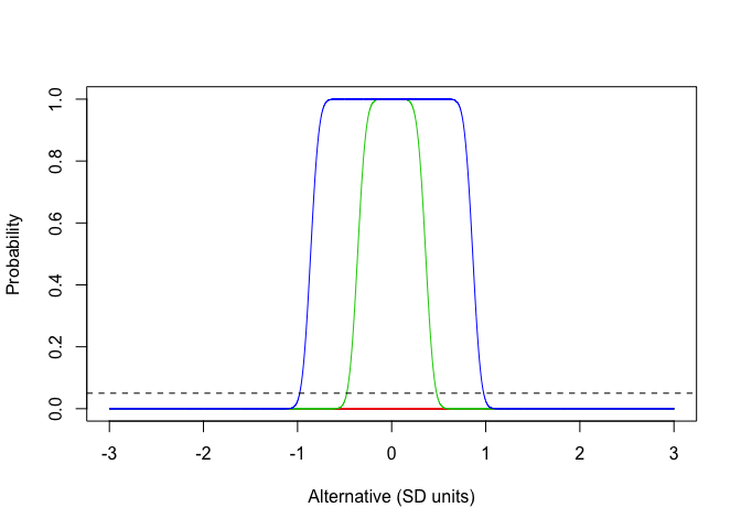
power_curves(delta = c(0, 1/30, 1/2, 1), n = 200, prob = "alternative")

Figure S6 from the second generation P-value paper. The relationship between the probability of an inconclusive result and various deltas.

## n = 20 (Figure S6 left)
power_curves(delta = c(0, 1/30, 1/2, 1), n = 20, prob = "inconclusive")

## n = 200 (Figure S6 right)
power_curves(delta = c(0, 1/30, 1/2, 1), n = 200, prob = "inconclusive")