Michael F. Gensheimer and Balasubramanian Narasimhan
Stanford University
mgens@stanford.edu
Keras version is compatible with Python version 3.7+ and TensorFlow version 2.0+.
PyTorch version is compatible with Python version 3.10+ and PyTorch version 2.2+.
nnet_survival.py: Keras version of Nnet-survival functions
nnet_survival_examples.py: Examples of use of Nnet-survival
nnet_survival_pytorch.py: PyTorch version of Nnet-survival functions
nnet_survival_pytorch_example.ipynb: Simple example of use of PyTorch version of Nnet-survival
support_study.py: Application of Nnet-survival to SUPPORT study data
Issues with Brown et al. 1997 loss function
Load libraries, including nnet_survival:
import numpy as np
import matplotlib.pyplot as plt
import matplotlib
from tensorflow.keras.models import Sequential, Model
from tensorflow.keras import optimizers, layers, regularizers
from tensorflow.keras.callbacks import EarlyStopping, ModelCheckpoint
from tensorflow.keras.layers import Input, Dense, Activation
from tensorflow.keras.models import load_model
from lifelines import KaplanMeierFitter
from lifelines import CoxPHFitter
from lifelines.utils import concordance_index
import nnet_survival
Create 39 equally spaced intervals for follow-up time, from 0 to 5 years:
breaks=np.arange(0.,365.*5,365./8)
n_intervals=len(breaks)-1
timegap = breaks[1:] - breaks[:-1]
Create data for 5000 simulated patients. There is one covariate (call it x). The first half of the patients have x=0, and have exponential survival distribution with half-life 200 days. The second half of the patients have x=1, and have exponential survival distribution with half-life 400 days. Some patients are censored, with censoring half-life of 400 days.
halflife1 = 200
halflife2 = 400
halflife_cens = 400
n_samples=5000
np.random.seed(seed=0)
t1 = np.random.exponential(scale=1 / (np.log(2)/halflife1), size=int(n_samples/2))
t2 = np.random.exponential(scale=1 / (np.log(2)/halflife2), size=int(n_samples/2))
t=np.concatenate((t1, t2))
censtime = np.random.exponential(scale=1 / (np.log(2)/(halflife_cens)), size=n_samples)
f = t<censtime
t[~f] = censtime[~f]
x_train = np.zeros(n_samples)
x_train[int(n_samples/2):]=1
Convert each patient's output data from (time, censoring indicator) format to a vector that for each time interval specifies whether the patient survived that time interval, and whether the patient failed during that time interval:
y_train=nnet_survival.make_surv_array(t,f,breaks)Train model, usuing a custom Keras loss function called surv_likelihood. For each time interval, a separate hazard rate is estimated.
model = Sequential()
#Hidden layers would go here. For this example, using simple linear model with no hidden layers.
model.add(Dense(n_intervals,input_dim=1, kernel_initializer='zeros', bias_initializer='zeros'))
model.add(Activation('sigmoid'))
model.compile(loss=nnet_survival.surv_likelihood(n_intervals), optimizer=optimizers.RMSprop())
#model.summary()
early_stopping = EarlyStopping(monitor='loss', patience=2)
history=model.fit(x_train, y_train, batch_size=256, epochs=1000, callbacks=[early_stopping])
y_pred=model.predict_proba(x_train,verbose=0)
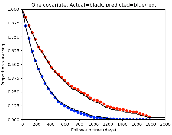
For each of the two groups, plot true survival distribution (Kaplan-Meier estimator) and compare to model-predicted survival.
kmf = KaplanMeierFitter()
kmf.fit(t[0:int(n_samples/2)], event_observed=f[0:int(n_samples/2)])
plt.plot(breaks,np.concatenate(([1],np.cumprod(y_pred[0,:]))),'bo-')
plt.plot(kmf.survival_function_.index.values, kmf.survival_function_.KM_estimate,color='k')
kmf.fit(t[int(n_samples/2)+1:], event_observed=f[int(n_samples/2)+1:])
plt.plot(breaks,np.concatenate(([1],np.cumprod(y_pred[-1,:]))),'ro-')
plt.plot(kmf.survival_function_.index.values, kmf.survival_function_.KM_estimate,color='k')
plt.xticks(np.arange(0, 2000.0001, 200))
plt.yticks(np.arange(0, 1.0001, 0.125))
plt.xlim([0,2000])
plt.ylim([0,1])
plt.xlabel('Follow-up time (days)')
plt.ylabel('Proportion surviving')
plt.title('One covariate. Actual=black, predicted=blue/red.')
plt.show()
The model has good agreement with the true survival distribution:
It is easy to output a predicted survival curve for an individual, or a predicted survival probability at a specific follow-up time. For instance, print the predicted survival probability for the 100th individual at a follow-up time of 30 days:
pred_surv = nnet_survival.nnet_pred_surv(model.predict_proba(x_train,verbose=0), breaks, 30)
print(pred_surv[99])