spatialrisk is a R-package for spatial risk calculations. It offers an
efficient approach to determine the sum of all observations within a
circle of a certain radius. This might be beneficial for insurers who
are required (by a recent European Commission regulation) to determine
the maximum value of insured fire risk policies of all buildings that
are partly or fully located within a circle of a radius of 200m. The key
functions in spatialrisk are written in C++ (using Rcpp), and are
therefore very fast.
Install spatialrisk from CRAN:
install.packages("spatialrisk")Or the development version from GitHub:
# install.packages("remotes")
remotes::install_github("MHaringa/spatialrisk")Filter all observations in Groningen that fall within a circle of a
radius of 100m drawn around the point (lon,lat) = (6.561561,53.21326):
library(spatialrisk)
circle <- points_in_circle(Groningen, lon_center = 6.571561, lat_center = 53.21326, radius = 100)
circle
## # A tibble: 14 × 10
## street number letter suffix postal_code city lon lat amount distance_m
## <chr> <int> <chr> <chr> <chr> <chr> <dbl> <dbl> <dbl> <dbl>
## 1 Heresin… 5 <NA> <NA> 9711EP Gron… 6.57 53.2 5 31.4
## 2 Heresin… 11 <NA> <NA> 9711ER Gron… 6.57 53.2 11 47.8
## 3 Zuiderp… 1003 <NA> <NA> 9724AK Gron… 6.57 53.2 1003 57.6
## 4 Heresin… 13 <NA> <NA> 9711ER Gron… 6.57 53.2 13 68.1
## 5 Hereple… 10 <NA> <NA> 9711GA Gron… 6.57 53.2 10 74.6
## 6 Heresin… 16 <NA> <NA> 9711ES Gron… 6.57 53.2 16 84.1
## 7 Heresin… 6 <NA> <NA> 9711ES Gron… 6.57 53.2 6 86.2
## 8 Heresin… 6 a <NA> 9711ES Gron… 6.57 53.2 6 87.8
## 9 Heresin… 6 b <NA> 9711ES Gron… 6.57 53.2 6 90.9
## 10 Heresin… 20 <NA> <NA> 9711ET Gron… 6.57 53.2 20 91.5
## 11 Heresin… 20 a <NA> 9711ET Gron… 6.57 53.2 20 93.0
## 12 Heresin… 15 a <NA> 9711ER Gron… 6.57 53.2 15 95.1
## 13 Zuiderp… 1007 <NA> <NA> 9724AK Gron… 6.57 53.2 1007 97.2
## 14 Zuiderp… 25 a <NA> 9724AJ Gron… 6.57 53.2 25 97.8
The sum of all observations within this circle is equal to:
sum(circle$amount)## [1] 2163
The next example shows how to determine the sum of all observations within a circle with a certain radius for multiple points.
concentration() determines the sum of all observations within a circle
of a certain radius for multiple points. Find for each row in df the
sum of all observations in Groningen within a circle of a radius of
100m from the (lon,lat) pair:
df <- data.frame(location = c("p1", "p2", "p3"),
                 lon = c(6.561561, 6.561398, 6.571561),
                 lat = c(53.21369, 53.21326, 53.21326))

conc <- concentration(df, Groningen, value = amount, radius = 100)
conc
## location lon lat concentration
## 1 p1 6.561561 53.21369 775
## 2 p2 6.561398 53.21326 2271
## 3 p3 6.571561 53.21326 2163
Show that result is indeed equal to the result from Example 1:
isTRUE(sum(circle$amount) == conc$concentration[3])## [1] TRUE
Example 2 shows how to determine the sum of all observations within a
circle of certain radius for multiple points.
find_highest_concentration() can be used to determine the central
coordinates of a circle with a constant radius that maximizes the
coverage of demand points. As an example this is applied to data set
Groningen.
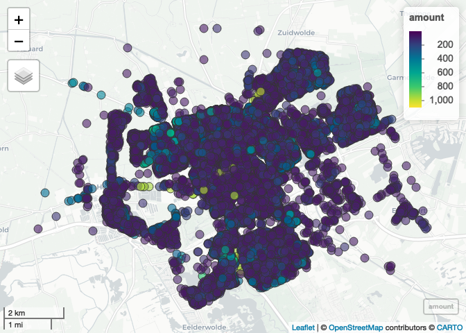
Show all points in data set Groningen:
plot_points(Groningen, value = "amount")Find the central coordinates of a circle with the highest concentration:
hconc <- find_highest_concentration(Groningen,
                                    value = "amount",
                                    radius = 200)
## Time difference of 0.4750721 secs
Note that all functions are written in C++, and are therefore very fast.
Output highest concentration:
hc[[1]]## lon lat concentration cell id
## 1 6.547326 53.23658 64438 3642 1
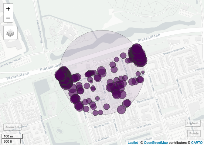
Plot the points in the highest concentration highest concentration. The sum of all values is equal to the concentration. This concentration is the highest in data set Groningen.
Show the highest concentration on a map (the highest concentration includes two apartment buildings with many objects):
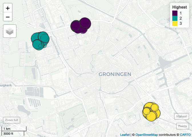
plot(hc)Its also possible to show the coordinates for more than one concentration. To show the second and third highest concentration:
hconc <- find_highest_concentration(Groningen,
                                    value = "amount",
                                    radius = 200,
                                    top_n = 3)
## Finished 1 of 3Finished 2 of 3Finished 3 of 3
Create interactive map:
plot(hconc)Show objects in the highest circle:
hc[[2]]## # A tibble: 208 × 13
## street number letter suffix postal_code city lon lat amount ix
## <chr> <int> <chr> <chr> <chr> <chr> <dbl> <dbl> <dbl> <int>
## 1 Elzenlaan 135 <NA> <NA> 9741ND Gron… 6.55 53.2 135 20449
## 2 Elzenlaan 139 <NA> <NA> 9741ND Gron… 6.55 53.2 139 23229
## 3 Elzenlaan 70 <NA> <NA> 9741NG Gron… 6.55 53.2 70 585
## 4 Elzenlaan 68 <NA> <NA> 9741NG Gron… 6.55 53.2 68 14677
## 5 Duindoornstr… 1 <NA> <NA> 9741NM Gron… 6.55 53.2 12 16828
## 6 Duindoornstr… 17 <NA> <NA> 9741NM Gron… 6.55 53.2 17 12829
## 7 Duindoornstr… 15 <NA> <NA> 9741NM Gron… 6.55 53.2 15 16004
## 8 Duindoornstr… 21 <NA> <NA> 9741NM Gron… 6.55 53.2 21 11748
## 9 Duindoornstr… 13 <NA> <NA> 9741NM Gron… 6.55 53.2 13 2006
## 10 Ranonkelstra… 38 <NA> <NA> 9741LT Gron… 6.55 53.2 38 19696
## # ℹ 198 more rows
## # ℹ 3 more variables: distance_m <dbl>, id <int>, conc <dbl>
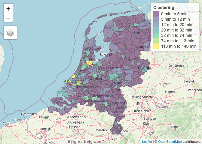
spatialrisk also contains functionality to create choropleths.
Typically in R it is difficult to create choropleths.
points_to_polygon() attempts to elegantly solve this problem.
The common approach is to first aggregate the data on the level of the
regions in the shapefile, and then merging the aggregated data with the
shapefile. Despite it being common, it is problematic in case the names
in the data and the names in the shapefile do not match. This is for
example the case when there are differences in punctuation marks in the
area names. Therefore, points_to_polygon() uses the longitude and
latitude of a point to map this point to a region. This approach makes
it easy to create choropleth maps on different region levels.
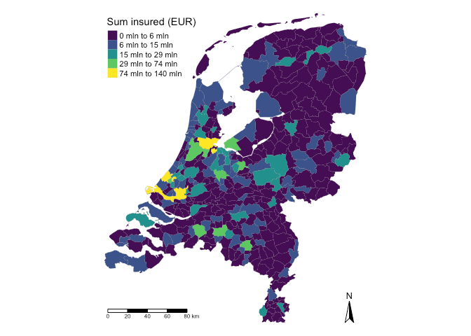
This example shows how points_to_polygon() is used to map the total
sum insured on the municipality level in the Netherlands:
gemeente_sf <- points_to_polygon(nl_gemeente, insurance, sum(amount, na.rm = TRUE))choropleth() creates a map based on the simple feature object obtained
in the previous step. There are two options to create a choropleth map.
When mode is set to plot a static map is created. The given
clustering is according to the Fisher-Jenks algorithm. This commonly
used classification method for choropleths seeks to reduce the variance
within classes and maximize the variance between classes.
choropleth(gemeente_sf, mode = "plot", legend_title = "Sum insured (EUR)", n = 5)If mode is set to view an interactive map is created:
choropleth(gemeente_sf, mode = "view", legend_title = "Sum insured (EUR)")The following simple feature objects are available in spatialrisk:
nl_provincie, nl_corop, nl_gemeente, nl_postcode1,
nl_postcode2, nl_postcode3, nl_postcode4, world_countries, and
europe_countries.
