pyBreakDown

Please note that the Break Down method is moved to the dalex Python package which is actively maintained. If you will experience any problem with pyBreakDown please consider the dalex implementation at https://dalex.drwhy.ai/python/api/.

Python implementation of breakDown package (https://github.com/pbiecek/breakDown).

Docs: https://pybreakdown.readthedocs.io.

Requirements

Nothing fancy, just python 3.5.2+ and pip.

Installation

Install directly from github

    git clone https://github.com/bondyra/pyBreakDown
    cd ./pyBreakDown
    python3 setup.py install  # (or use pip install . instead)

Basic usage

Load dataset

from sklearn import datasets

x = datasets.load_boston()

data = x.data

feature_names = x.feature_names

y = x.target

Prepare model

import numpy as np

from sklearn import tree

model = tree.DecisionTreeRegressor()

Train model

train_data = data[1:300,:]
train_labels=y[1:300]

model = model.fit(train_data,y=train_labels)

Explain predictions on test data

#necessary imports
from pyBreakDown.explainer import Explainer
from pyBreakDown.explanation import Explanation

#make explainer object
exp = Explainer(clf=model, data=train_data, colnames=feature_names)

#make explanation object that contains all information
explanation = exp.explain(observation=data[302,:],direction="up")

Text form of explanations

#get information in text form
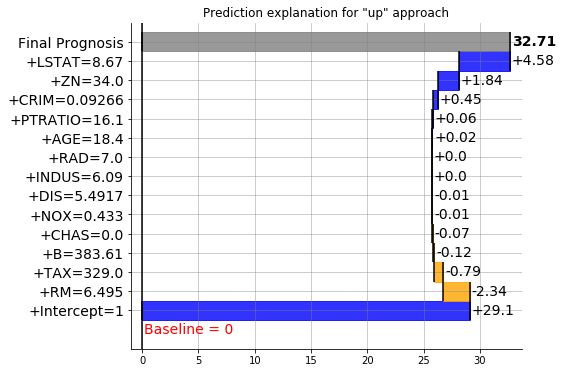
explanation.text()

Feature                  Contribution        Cumulative          
Intercept = 1            29.1                29.1                
RM = 6.495               -1.98               27.12               
TAX = 329.0              -0.2                26.92               
B = 383.61               -0.12               26.79               
CHAS = 0.0               -0.07               26.72               
NOX = 0.433              -0.02               26.7                
RAD = 7.0                0.0                 26.7                
INDUS = 6.09             0.01                26.71               
DIS = 5.4917             -0.04               26.66               
ZN = 34.0                0.01                26.67               
PTRATIO = 16.1           0.04                26.71               
AGE = 18.4               0.06                26.77               
CRIM = 0.09266           1.33                28.11               
LSTAT = 8.67             4.6                 32.71               
Final prediction                             32.71               
Baseline = 0

#customized text form
explanation.text(fwidth=40, contwidth=40, cumulwidth = 40, digits=4)

Feature                                 Contribution                            Cumulative                              
Intercept = 1                           29.1                                    29.1                                    
RM = 6.495                              -1.9826                                 27.1174                                 
TAX = 329.0                             -0.2                                    26.9174                                 
B = 383.61                              -0.1241                                 26.7933                                 
CHAS = 0.0                              -0.0686                                 26.7247                                 
NOX = 0.433                             -0.0241                                 26.7007                                 
RAD = 7.0                               0.0                                     26.7007                                 
INDUS = 6.09                            0.0074                                  26.708                                  
DIS = 5.4917                            -0.0438                                 26.6642                                 
ZN = 34.0                               0.0077                                  26.6719                                 
PTRATIO = 16.1                          0.0385                                  26.7104                                 
AGE = 18.4                              0.0619                                  26.7722                                 
CRIM = 0.09266                          1.3344                                  28.1067                                 
LSTAT = 8.67                            4.6037                                  32.7104                                 
Final prediction                                                                32.7104                                 
Baseline = 0

Visual form of explanations

explanation.visualize()

#customize height, width and dpi of plot
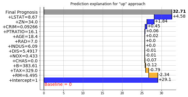
explanation.visualize(figsize=(8,5),dpi=100)

#for different baselines than zero
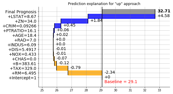
explanation = exp.explain(observation=data[302,:],direction="up",useIntercept=True)  # baseline==intercept
explanation.visualize(figsize=(8,5),dpi=100)

MI2DataLab/pyBreakDown