


The repository is for the development of neural network solvers of differential equations such as physics-informed neural networks (PINNs) and deep BSDE solvers. It utilizes techniques like deep neural networks and neural stochastic differential equations to make it practical to solve high dimensional PDEs efficiently through the likes of scientific machine learning (SciML).
julia ./install.jlIn this example we will solve a Hamilton-Jacobi-Bellman equation of 100 dimensions.
The Hamilton-Jacobi-Bellman equation is the solution to a stochastic optimal
control problem. Here, we choose to solve the classical Linear Quadratic Gaussian
(LQG) control problem of 100 dimensions, which is governed by the SDE
dX_t = 2sqrt(λ)c_t dt + sqrt(2)dW_t where c_t is a control process. The solution
to the optimal control is given by a PDE of the form:
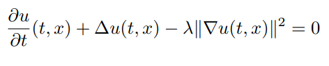
with terminating condition g(X) = log(0.5f0 + 0.5f0*sum(X.^2)). To solve it
using the TerminalPDEProblem, we write:
d = 100 # number of dimensions
X0 = fill(0.0f0,d) # initial value of stochastic control process
tspan = (0.0f0, 1.0f0)
λ = 1.0f0

g(X) = log(0.5f0 + 0.5f0*sum(X.^2))
f(X,u,σᵀ∇u,p,t) = -λ*sum(σᵀ∇u.^2)
μ_f(X,p,t) = zero(X)  #Vector d x 1 λ
σ_f(X,p,t) = Diagonal(sqrt(2.0f0)*ones(Float32,d)) #Matrix d x d
prob = TerminalPDEProblem(g, f, μ_f, σ_f, X0, tspan)
As described in the API docs, we now need to define our NNPDENS algorithm
by giving it the Flux.jl chains we want it to use for the neural networks.
u0 needs to be a d dimensional -> 1 dimensional chain, while σᵀ∇u
needs to be d+1 dimensional to d dimensions. Thus we define the following:
hls = 10 + d #hidden layer size
opt = Flux.ADAM(0.01)  #optimizer
#sub-neural network approximating solutions at the desired point
u0 = Flux.Chain(Dense(d,hls,relu),
                Dense(hls,hls,relu),
                Dense(hls,1))
# sub-neural network approximating the spatial gradients at time point
σᵀ∇u = Flux.Chain(Dense(d+1,hls,relu),
                  Dense(hls,hls,relu),
                  Dense(hls,hls,relu),
                  Dense(hls,d))
pdealg = NNPDENS(u0, σᵀ∇u, opt=opt)
And now we solve the PDE. Here we say we want to solve the underlying neural
SDE using the Euler-Maruyama SDE solver with our chosen dt=0.2, do at most
100 iterations of the optimizer, 100 SDE solves per loss evaluation (for averaging),
and stop if the loss ever goes below 1f-2.
@time ans = solve(prob, pdealg, verbose=true, maxiters=100, trajectories=100,
                            alg=EM(), dt=0.2, pabstol = 1f-2)
In this example we will solve a Black-Scholes-Barenblatt equation of 100 dimensions. The Black-Scholes-Barenblatt equation is a nonlinear extension to the Black-Scholes equation which models uncertain volatility and interest rates derived from the Black-Scholes equation. This model results in a nonlinear PDE whose dimension is the number of assets in the portfolio.
To solve it using the TerminalPDEProblem, we write:
d = 100 # number of dimensions
X0 = repeat([1.0f0, 0.5f0], div(d,2)) # initial value of stochastic state
tspan = (0.0f0,1.0f0)
r = 0.05f0
sigma = 0.4f0
f(X,u,σᵀ∇u,p,t) = r * (u - sum(X.*σᵀ∇u))
g(X) = sum(X.^2)
μ_f(X,p,t) = zero(X) #Vector d x 1
σ_f(X,p,t) = Diagonal(sigma*X) #Matrix d x d
prob = TerminalPDEProblem(g, f, μ_f, σ_f, X0, tspan)
As described in the API docs, we now need to define our NNPDENS algorithm
by giving it the Flux.jl chains we want it to use for the neural networks.
u0 needs to be a d dimensional -> 1 dimensional chain, while σᵀ∇u
needs to be d+1 dimensional to d dimensions. Thus we define the following:
hls  = 10 + d #hide layer size
opt = Flux.ADAM(0.001)
u0 = Flux.Chain(Dense(d,hls,relu),
                Dense(hls,hls,relu),
                Dense(hls,1))
σᵀ∇u = Flux.Chain(Dense(d+1,hls,relu),
                  Dense(hls,hls,relu),
                  Dense(hls,hls,relu),
                  Dense(hls,d))
pdealg = NNPDENS(u0, σᵀ∇u, opt=opt)
And now we solve the PDE. Here we say we want to solve the underlying neural
SDE using the Euler-Maruyama SDE solver with our chosen dt=0.2, do at most
150 iterations of the optimizer, 100 SDE solves per loss evaluation (for averaging),
and stop if the loss ever goes below 1f-6.
ans = solve(prob, pdealg, verbose=true, maxiters=150, trajectories=100,
alg=EM(), dt=0.2, pabstol = 1f-6)To solve high dimensional PDEs, first one should describe the PDE in terms of
the TerminalPDEProblem with constructor:
TerminalPDEProblem(g,f,μ_f,σ_f,X0,tspan,p=nothing)which describes the semilinear parabolic PDE of the form:
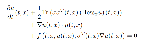
with terminating condition u(tspan[2],x) = g(x). These methods solve the PDE in
reverse, satisfying the terminal equation and giving a point estimate at
u(tspan[1],X0). The dimensionality of the PDE is determined by the choice
of X0, which is the initial stochastic state.
To solve this PDE problem, there exists two algorithms:
NNPDENS(u0,σᵀ∇u;opt=Flux.ADAM(0.1)): Uses a neural stochastic differential equation which is then solved by the methods available in DifferentialEquations.jl Thealgkeyword is required for specifying the SDE solver algorithm that will be used on the internal SDE. All of the other keyword arguments are passed to the SDE solver.NNPDEHan(u0,σᵀ∇u;opt=Flux.ADAM(0.1)): Uses the stochastic RNN algorithm from Han. Only applicable whenμ_fandσ_fresult in a non-stiff SDE where low order non-adaptive time stepping is applicable.
Here, u0 is a Flux.jl chain with d dimensional input and 1 dimensional output.
For NNPDEHan, σᵀ∇u is an array of M chains with d dimensional input and
d dimensional output, where M is the total number of timesteps. For NNPDENS
it is a d+1 dimensional input (where the final value is time) and d dimensional
output. opt is a Flux.jl optimizer.
Each of these methods has a special keyword argument pabstol which specifies
an absolute tolerance on the PDE's solution, and will exit early if the loss
reaches this value. Its defualt value is 1f-6.
For ODEs, see the DifferentialEquations.jl documentation
for the nnode(chain,opt=ADAM(0.1)) algorithm, which takes in a Flux.jl chain
and optimizer to solve an ODE. This method is not particularly efficient, but
is parallel. It is based on the work of:
A Kolmogorov PDE is of the form :

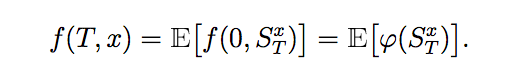
Considering S be a solution process to the SDE:
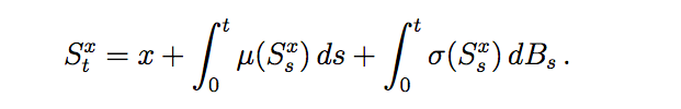
then the solution to the Kolmogorov PDE is given as:
A Kolmogorov PDE Problem can be defined using a SDEProblem:
SDEProblem(μ,σ,u0,tspan,xspan,d)Here u0 is the initial distribution of x. Here we define u(0,x) as the probability density function of u0.μ and σ are obtained from the SDE for the stochastic process above. d represents the dimenstions of x.
u0 can be defined using Distributions.jl.
Another was of defining a KolmogorovPDE is using the KolmogorovPDEProblem.
KolmogorovPDEProblem(μ,σ,phi,tspan,xspan,d)Here phi is the initial condition on u(t,x) when t = 0. μ and σ are obtained from the SDE for the stochastic process above. d represents the dimenstions of x.
To solve this problem use,
NNKolmogorov(chain, opt , sdealg): Uses a neural network to realise a regression function which is the solution for the linear Kolmogorov Equation.
Here, chain is a Flux.jl chain with d dimensional input and 1 dimensional output.opt is a Flux.jl optimizer. And sdealg is a high-order algorithm to calculate the solution for the SDE, which is used to define the learning data for the problem. Its default value is the classic Euler-Maruyama algorithm.
- ReservoirComputing.jl has an implementation of the Echo State Network method for learning the attractor properties of a chaotic system.