The goal of veganomics is to provide extra functions for using vegan with -omics data such as RNA-Seq or microarrays, including functions for:
- Filtering, normalizing and scaling expression matrices for use with rda()
- Improved plotting of variance partioning between constrained/non-constrained components from rda()
- Improved plotting of study design and sample strain from rda()
Some functions also work for cca()
You can install the development version of veganomics from GitHub with:
# install.packages("devtools")
devtools::install_github("MalteThodberg/veganomics")The following includes some example analysis using various datasets from Bioconductor.
library(veganomics)
#> Loading required package: ggplot2
#> Loading required package: patchwork
#> Loading required package: vegan
#> Loading required package: permute
#> Loading required package: lattice
#> This is vegan 2.6-4
theme_set(theme_bw())# Data
library(SummarizedExperiment)
#> Loading required package: MatrixGenerics
#> Loading required package: matrixStats
#>
#> Attaching package: 'MatrixGenerics'
#> The following objects are masked from 'package:matrixStats':
#>
#> colAlls, colAnyNAs, colAnys, colAvgsPerRowSet, colCollapse,
#> colCounts, colCummaxs, colCummins, colCumprods, colCumsums,
#> colDiffs, colIQRDiffs, colIQRs, colLogSumExps, colMadDiffs,
#> colMads, colMaxs, colMeans2, colMedians, colMins, colOrderStats,
#> colProds, colQuantiles, colRanges, colRanks, colSdDiffs, colSds,
#> colSums2, colTabulates, colVarDiffs, colVars, colWeightedMads,
#> colWeightedMeans, colWeightedMedians, colWeightedSds,
#> colWeightedVars, rowAlls, rowAnyNAs, rowAnys, rowAvgsPerColSet,
#> rowCollapse, rowCounts, rowCummaxs, rowCummins, rowCumprods,
#> rowCumsums, rowDiffs, rowIQRDiffs, rowIQRs, rowLogSumExps,
#> rowMadDiffs, rowMads, rowMaxs, rowMeans2, rowMedians, rowMins,
#> rowOrderStats, rowProds, rowQuantiles, rowRanges, rowRanks,
#> rowSdDiffs, rowSds, rowSums2, rowTabulates, rowVarDiffs, rowVars,
#> rowWeightedMads, rowWeightedMeans, rowWeightedMedians,
#> rowWeightedSds, rowWeightedVars
#> Loading required package: GenomicRanges
#> Loading required package: stats4
#> Loading required package: BiocGenerics
#>
#> Attaching package: 'BiocGenerics'
#> The following objects are masked from 'package:stats':
#>
#> IQR, mad, sd, var, xtabs
#> The following objects are masked from 'package:base':
#>
#> anyDuplicated, aperm, append, as.data.frame, basename, cbind,
#> colnames, dirname, do.call, duplicated, eval, evalq, Filter, Find,
#> get, grep, grepl, intersect, is.unsorted, lapply, Map, mapply,
#> match, mget, order, paste, pmax, pmax.int, pmin, pmin.int,
#> Position, rank, rbind, Reduce, rownames, sapply, setdiff, sort,
#> table, tapply, union, unique, unsplit, which.max, which.min
#> Loading required package: S4Vectors
#>
#> Attaching package: 'S4Vectors'
#> The following object is masked from 'package:utils':
#>
#> findMatches
#> The following objects are masked from 'package:base':
#>
#> expand.grid, I, unname
#> Loading required package: IRanges
#> Loading required package: GenomeInfoDb
#> Loading required package: Biobase
#> Welcome to Bioconductor
#>
#> Vignettes contain introductory material; view with
#> 'browseVignettes()'. To cite Bioconductor, see
#> 'citation("Biobase")', and for packages 'citation("pkgname")'.
#>
#> Attaching package: 'Biobase'
#> The following object is masked from 'package:MatrixGenerics':
#>
#> rowMedians
#> The following objects are masked from 'package:matrixStats':
#>
#> anyMissing, rowMedians
library(bladderbatch)
data("bladderdata")
# Convert from eSet to SummarizedExperiment and format a bit
SE <- as(bladderEset, "SummarizedExperiment")
SE$batch <- factor(SE$batch) |> forcats::fct_infreq()
SE$cancer <- relevel(SE$cancer, "Normal")
# Normalize
EM <- t(assay(SE))
# Simple PCA
fit_pca <- rda(EM, scale=TRUE)
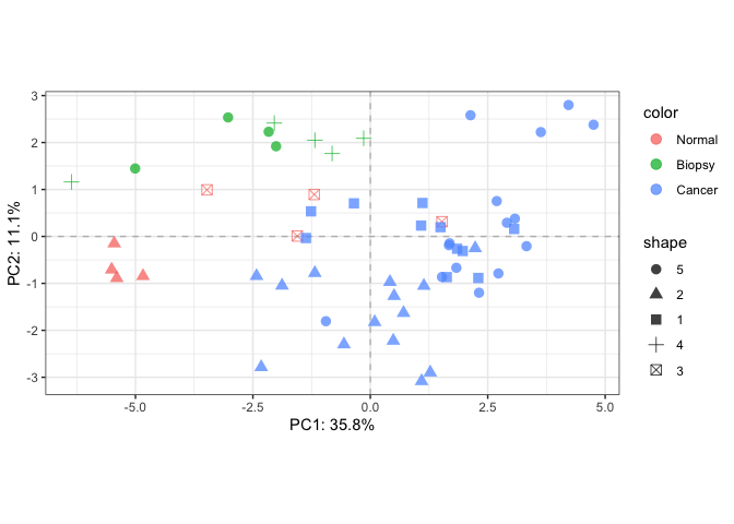
plotTotal(fit_pca, color=SE$cancer, shape=SE$batch)# Fit RDA
fit_rda <- rda(formula=EM~outcome,
data=as.data.frame(colData(SE)), scale=TRUE)
# Visualize decomposition
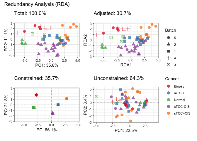
plotDecomposition(fit_rda,
color=SE$outcome,
shape=SE$batch,
color_scale = scale_color_brewer("Cancer", palette = "Set1"),
shape_scale = scale_shape("Batch"))
#> Refitting PCA...# Further inspect model
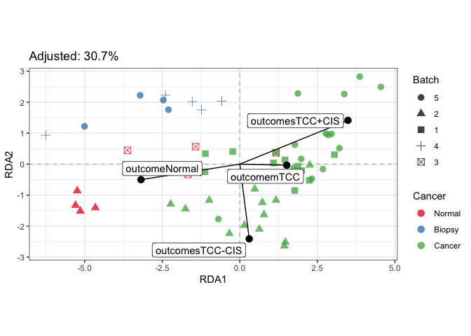
plotDesign(fit_rda, color=SE$cancer, shape=SE$batch) +
scale_color_brewer("Cancer", palette = "Set1") +
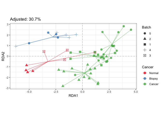
scale_shape("Batch")plotStrain(fit_rda, color=SE$cancer, shape=SE$batch) +
scale_color_brewer("Cancer", palette = "Set1") +
scale_shape("Batch")# Example of corresponding tests in vegan
anova(fit_rda,
permutations = how(nperm=99), # SET THIS TOO ATLEAST 999!!!
by="term")
#> Permutation test for rda under reduced model
#> Terms added sequentially (first to last)
#> Permutation: free
#> Number of permutations: 99
#>
#> Model: rda(formula = EM ~ outcome, data = as.data.frame(colData(SE)), scale = TRUE)
#> Df Variance F Pr(>F)
#> outcome 4 7948 7.2078 0.01 **
#> Residual 52 14335
#> ---
#> Signif. codes: 0 '***' 0.001 '**' 0.01 '*' 0.05 '.' 0.1 ' ' 1
anova(fit_rda,
permutations = how(nperm=99), # SET THIS TOO ATLEAST 999!!!
by="axis")
#> Permutation test for rda under reduced model
#> Forward tests for axes
#> Permutation: free
#> Number of permutations: 99
#>
#> Model: rda(formula = EM ~ outcome, data = as.data.frame(colData(SE)), scale = TRUE)
#> Df Variance F Pr(>F)
#> RDA1 1 5250.0 19.0445 0.01 **
#> RDA2 1 1728.9 6.2717 0.01 **
#> RDA3 1 646.9 2.3465 0.04 *
#> RDA4 1 322.2 1.1686 0.27
#> Residual 52 14335.0
#> ---
#> Signif. codes: 0 '***' 0.001 '**' 0.01 '*' 0.05 '.' 0.1 ' ' 1library(parathyroidSE)
data("parathyroidGenesSE")
# Filter counts using edgeR
CM <- filterCounts(~treatment*time,
data=colData(parathyroidGenesSE),
y=assay(parathyroidGenesSE))
# Normalize
EM <- normalizeCounts(CM)
# Simple PCA
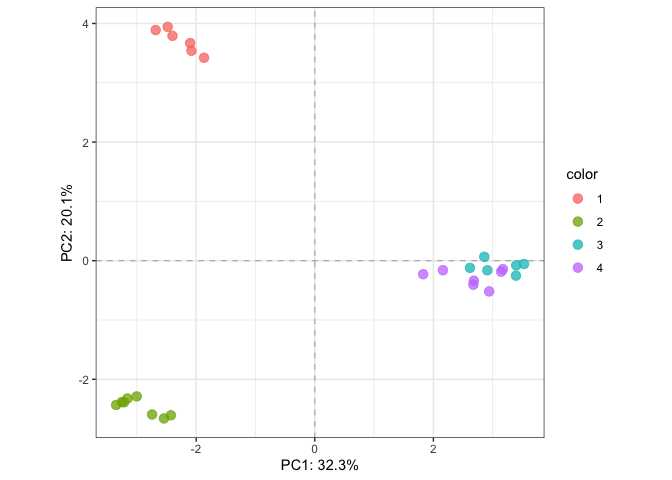
fit_pca <- rda(EM, scale=TRUE)
plotTotal(fit_pca, color=parathyroidGenesSE$patient)# RDA
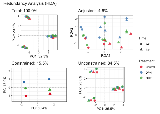
fit_rda <- rda(formula=EM~treatment*time,
data=as.data.frame(colData(parathyroidGenesSE)), scale=TRUE)
# Visualize decomposition
plotDecomposition(fit_rda, color=parathyroidGenesSE$treatment, shape=parathyroidGenesSE$time,
color_scale = scale_color_brewer("Treatment", palette = "Set1"),
shape_scale = scale_shape("Time"))
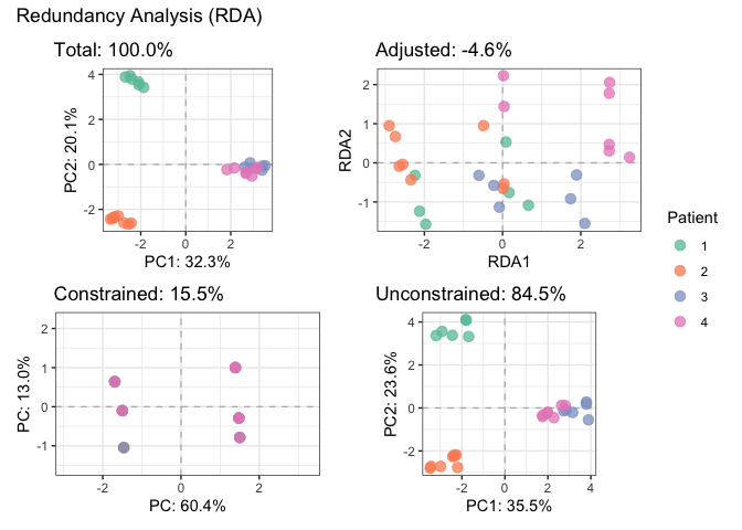
#> Refitting PCA...# Highligh batch effect
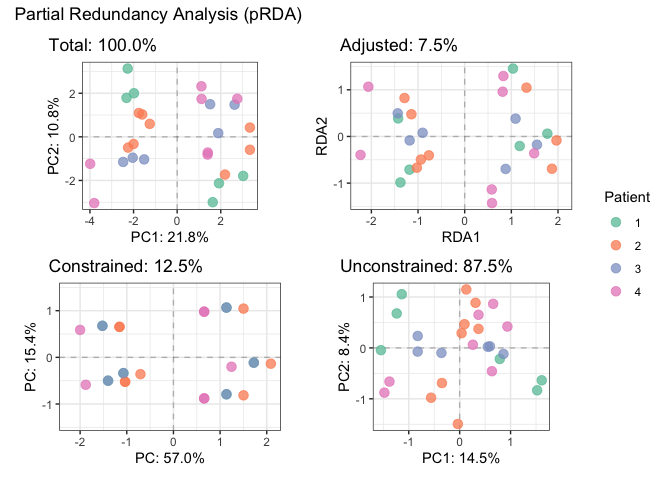
plotDecomposition(fit_rda, color=parathyroidGenesSE$patient,
color_scale = scale_color_brewer("Patient", palette = "Set2"))
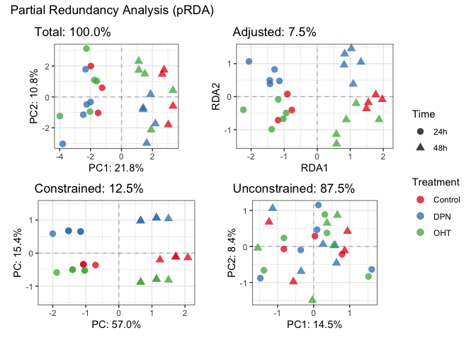
#> Refitting PCA...# Fit partial RDA to remove batch effect
fit_prda <- rda(formula=EM~treatment+time+treatment:time+Condition(patient),
data=as.data.frame(colData(parathyroidGenesSE)), scale=TRUE)
# Corrected
plotDecomposition(fit_prda, color=parathyroidGenesSE$treatment, shape=parathyroidGenesSE$time,
color_scale = scale_color_brewer("Treatment", palette = "Set1"),
shape_scale = scale_shape("Time"))
#> Refitting PCA...plotDecomposition(fit_prda, color=parathyroidGenesSE$patient,
color_scale = scale_color_brewer("Patient", palette = "Set2"))
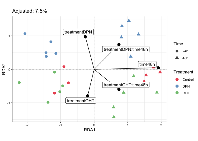
#> Refitting PCA...# Further introspection of pRDA
plotDesign(fit_prda, color=parathyroidGenesSE$treatment, shape=parathyroidGenesSE$time) +
scale_color_brewer("Treatment", palette = "Set1") +
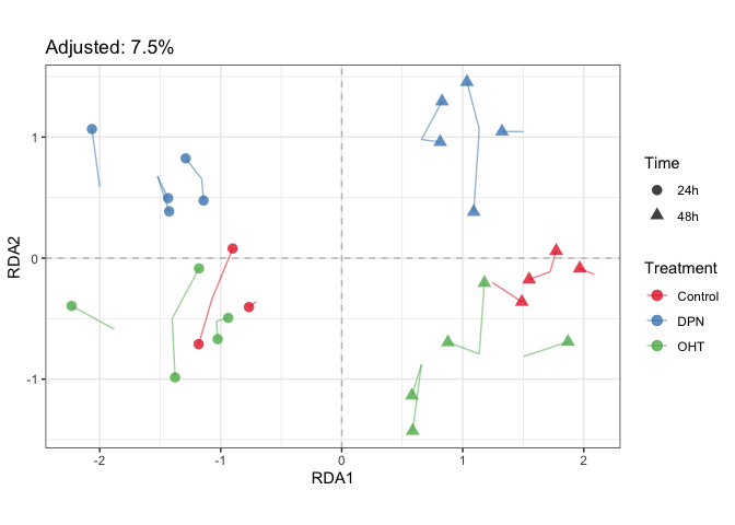
scale_shape("Time")plotStrain(fit_prda, color=parathyroidGenesSE$treatment, shape=parathyroidGenesSE$time) +
scale_color_brewer("Treatment", palette = "Set1") +
scale_shape("Time")# Test significance of terms
anova(fit_prda,
permutations = how(nperm=99), # SET THIS TOO ATLEAST 999!!!
by="term")
#> Permutation test for rda under reduced model
#> Terms added sequentially (first to last)
#> Permutation: free
#> Number of permutations: 99
#>
#> Model: rda(formula = EM ~ treatment + time + treatment:time + Condition(patient), data = as.data.frame(colData(parathyroidGenesSE)), scale = TRUE)
#> Df Variance F Pr(>F)
#> treatment 2 587.7 1.4934 0.07 .
#> time 1 1122.9 5.7069 0.01 **
#> treatment:time 2 372.0 0.9452 0.55
#> Residual 18 3541.7
#> ---
#> Signif. codes: 0 '***' 0.001 '**' 0.01 '*' 0.05 '.' 0.1 ' ' 1