output: github_document

rockr

The (current) goal of rockr is to identify top ranked bands from polling data on best album of the year. Given a series of Twitter polls on best album of the year, with sequential polls for each year, where some bands are reoccurring response options across polls, I

Munge data into an analysis-ready format
Produce multiple scalings and subsets of data to permit different ways of conceptualising poll results
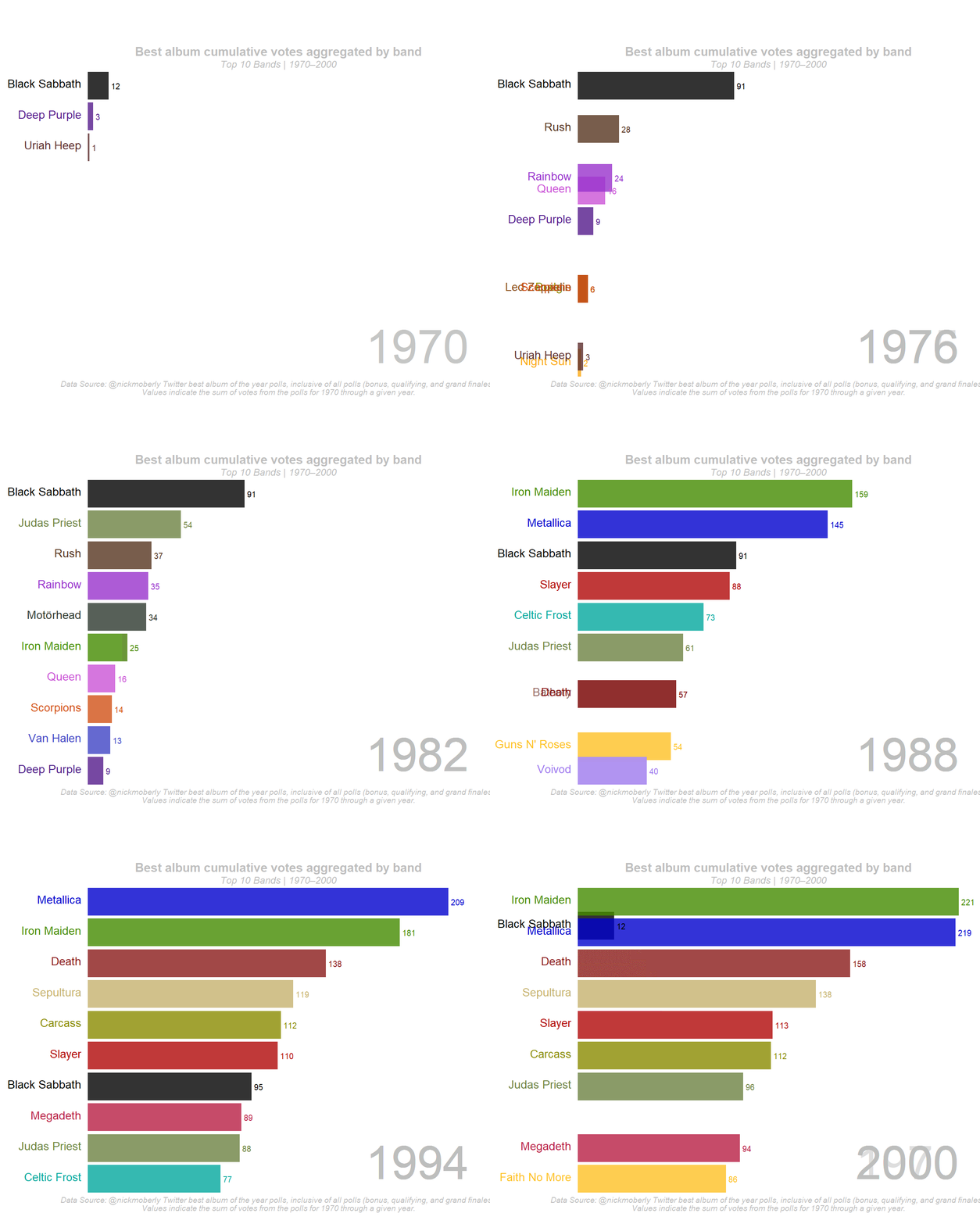
Render animated bar charts to visualise the cumulative and aggregate response across the series of polls

(Attempts at) British spelling are in honour of Nick Moberly (Exeter, UK), whose @nickmoberly Twitter polls were the motivation for and contributing data used in the illustrative example.

Packages, script, and data

Although rockr aspires to be a full blown package contributing an array of functions and analytic enhancements useful for a variety of applications, at present it is simply a code and data repository, with a script to perform one task, tailored to one particular dataset. See section, Future development of rockr, for thoughts on what rockr might be when it grows up.

The analyses described herein requires the installation and loading of the following R packages:

tidyverse, gt, gtsummary, install_phantomjs, ggplot2, gganimate, png

All R code required for this project can be found in R/twitter_api_poll_call.Rmd (for calling and cleaning the data) and R/Animated Bar Chart.Rmd (for analyzing and plotting the data), with raw data found in data-raw/raw_twitter_api_poll_data.csv

Analytic premises and assumptions (…however questionable)

A band’s status within the ranking of best bands is a function of
- the number of albums a band has that qualify as one of the best albums of the year and
- the proportion of people who vote a band’s albums as the best album of the year.
Poll percentages weighted equally across years smooths over variation in response rate across polls;
- however, the sum of votes may (in part) be an indicator of enthusiasm for a given band or album–and therefore may also be a valid metric for ranking bands.
  - polls for years 1984-1992 attracted more responses than earlier and later polls–perhaps signalling the best/most interesting era for metal.
Constraining the data to only the final poll for each year avoids the problem of needing to account for albums that appeared on both qualifying and final polls;
- however, on the premise that the magnitude of voter response is an indicator of enthusiasm for a given band or album, summing across bonus, qualifying, and final polls–constituting the total sum of votes cast for a band or album given the opportunity to vote for that band or album–may yield some insight.
Lastly, regarding these polls, it is worth noting that these are not scientifically derived samples–just Nick’s Twitter mates :)

Data preparation

Via access to the Twitter API, I used R programming to query and wrangle the poll data.

Regrettably, I have not devised a function that can call poll fields for an entire timeline all at once. Therefore, the procedure presented here required a first step of calling the conversation_ids for the entire timeline. Then, manually updating the Client URL in the code for each poll. This second step took 30-40 seconds for each call. Suggestions are welcome on a more elegant solution, such as a for()loop or lapply() function that cycles through the ids automatically.

Analysis file

Querying the Twitter API poll object returns data on the number of votes per poll response option, Accordingly, using the mutate() command I calculate the percentage of votes per response option.

Another preliminary step was to restructure the data to a long format using the pivot_longer() command to facilitate calculating summary statistics by survey id.

Exploration

The first thing I do is make a quick check for data error red flags. Using the group_by() and summarise(sum()) commands I calculate the sum of percentages for each response option for each poll; and using the mutate(sprintf()) and unique() commands to verify that all polls sum to 100 percent.

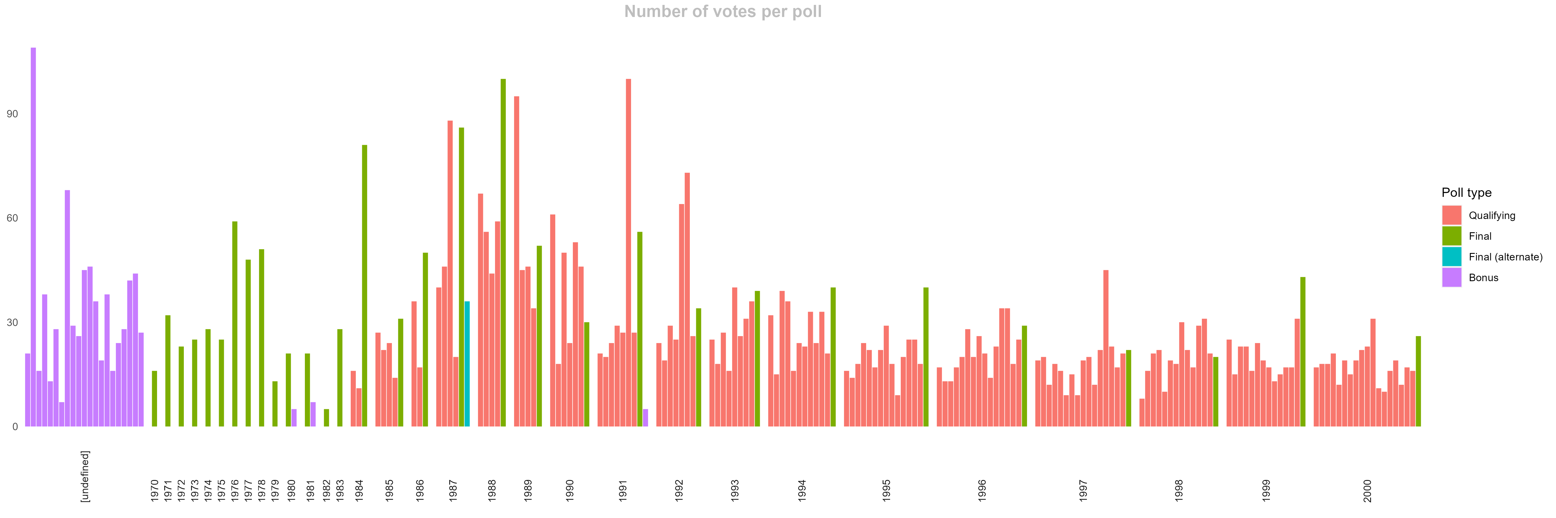
And using the ggplot() function, I produce a visualization to inspect the number of votes per poll. Here I use the facet_grid() command to group the polls for each album year.

I observe a suspiciously low number of votes for the 1982 final poll. Double-checking Twitter revealed that the 1982 poll indeed did have a low response rate: shocking given it included bangers such as Maiden’s Number of the Beast and Priest’s Screaming for Vengeance, making it clear that enthusiasm for the bands or albums can in no way explain all the variation in response rate.

Using the summarise(n_distinct()) command I see that across all qualifying and final polls, the data comprise 179 polls covering 247 bands cumulatively. Constraining to final polls only, the data comprise 31 polls covering 69 bands cumulatively.

Then, I use the tbl_summary() command to view the mean and standard deviation in poll votes by poll type to make some assessment of the central tendency and dispersion of responsiveness to the polls.

Selection

I then reduce the dataframe to the observations of interest.

For all analyses, I drop observations for polls coded as invalid.
- In the example data, one poll coded as invalid was conducted as an alternate final.
For two analyses I retain data for only final polls, excluding data for bonus and qualifying polls (see Bar Chart 1 and Bar Chart 2); for a third analysis I retained data for all valid polls, inclusive of bonus, qualifying, and final polls (see Bar Chart 3).

Aggregation

To remedy instances where a given band appeared more than once in a given year

I use the group_by() and summarise_at() commands to sum percentages or vote counts for each band per year.
This scenario occurred in the 1970 final poll, where Black Sabbath had two albums that year;
- other scenarios for this occur when analyzing bonus, qualifying, and final polls jointly.

Structure

Before undertaking the computations in the next step, I want a file in a long (tidy) format, with each band having a row for every year in the dataset regardless of whether the band had poll data for that year. There is probably a more efficient way of accomplishing this; but short of figuring that out,

I first used the pivot_wider() command, followed by the pivot_longer() command to accomplish this.
A more efficient approach might evaluate which years were unobserved for given bands, then insert rows for those missing observations.
- Suggestions on improved approaches to this are welcome.

Computation

To calculate rolling averages and sums, I use

the mutate(cummmean()) command with the poll_percent variable and
the mutate(cummsum()) command with the album_votes variable.

Format

The final step before plotting is to format the data for analysis by calling

the group_by() and mutate(rank()) commands to rank order the bands with each year and
the group_by() and filter() commands to constrain the data to the top ranked bands for any given year.
- In this example I filter to the top 10 ranked bands.

Rendering animated bar charts

Static and animated plots

The first step to making an animated bar chart is to plot a series of static bar charts using the ggplot() command.

Dissatisfied with the default colors, I create a custom array of colors and called it in using the scale_colour_manual() and scale_fill_manual() commands.
- After all, Black Sabbath has to be black and Deep Purple has to be purple, right?
Using the unique() command I can generate the list of bands in the plot for which colors are needed.

Then I use the transition_states() command to stitch together the individual static plots.

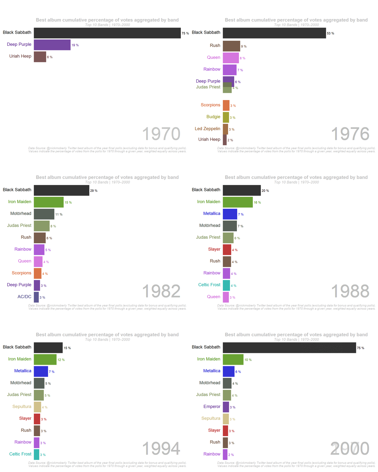
And the final step is rendering the animated plots using the animate(gifski_renderer()) command.

Bar Chart 1. Best album cumulative percentage of votes aggregated by band

This plot uses a rolling average of the poll_percent variable as the plotted metric, based on results according to the final polls.

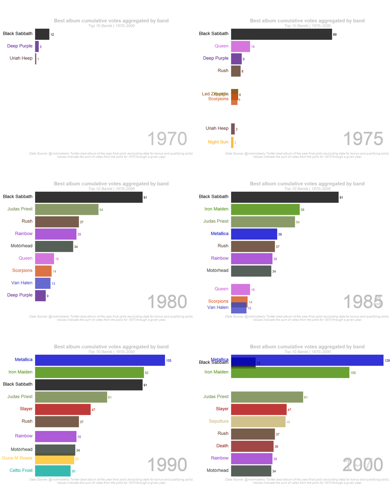
Bar Chart 2. Best album cumulative votes aggregated by band

This plot uses a rolling sum of the album_votes variable as the plotted metric, based on results according to the final polls.

This and the following plot that uses vote sums as the plotted metric has the annoying quirk of occasionally having ties where bars overlap–making the band name difficult to read.
- Suggested visualization remedies to the overlapping of bars are welcome.

Bar Chart 3. Best album cumulative votes aggregated by band

This plot uses a rolling sum of the album_votes variable as the plotted metric, based on results according to all polls.

Source code and guidance

Credit to AbdulMajedRaja RS for source code and guidance referenced for these animated bar charts. See also related Stack Overflow posts for guidance and discussion.

Future development of `rockr`

The most intuitive next step in development of rockr is to improve the method of calling poll fields from the Twitter API.
The exercise of deploying Twitter polls on album of the year derived from Nick’s (@NickMoberly) desire to fill gaps in knowledge on the prominent hard rock and metal bands over the decades. Accordingly, an enhancement to the function of rockr could be to integrate data that could be drawn upon for the purpose of informing the development of new polls and survey instruments.
- The Metal Archives: Encyclopdaedia Metallum is an extensive data repository on metal bands with information on home country, sub-genre, band members past and present, discography, related artists, etc.
  - JarbasAI’s Metal Dataset is an already conducted scraping of Metal Archives, though limited to only data on band names, song titles, and lyrics sorted by sub-genre. Incorporating these data would be an easy lift, though additional scraping of Metal Archives would be required to obtain data on discography, related artists, etc.
  - Then, using reactive programming, such as through R’s Shiny package, a dynamic user interface could be developed that draws upon the stores of data to generate lists of similar sets of bands or albums based on selected inputs.
    - In addition to facilitating poll development, the exercise of interacting with a rockr interface of this kind could in itself be a generative exercise for one’s own exploration.
      - Some of this functionality can already be accomplished through the many music streaming services available, except the UI described here would/could be more comprehensive in its directories, unimpeded by the various constraints with which those services contend around access and use.
Additional data that might be incorporated include archives of rankings according to rock and metal ’zine charts and reviews, including those from prominent outlets like Kerrang! and Metal Hammer, as well as smaller independent outlets and fanzines. Cult Never Dies, The Corroseum, Rare & Obscure Metal and Send Back My Stamps! are example webstores and repositories of metal fanzines that might be drawn upon, not to mention university archives that could be accessed.
- An extraordinarily ambitious undertaking might be to even incorporate text from interviews and articles published in such sources. The opportunities for textual analysis from such a data repository would be tremendous.
- A data repository of this kind would constitute a robust basis for clustering bands according to style and influence. Analytic approaches such as latent transition analyses and machine learning techniques could be leveraged to group bands by profile, allowing profile to vary over time according to observed indicators for albums.
Further, spotifyr, a R wrapper for Spotify’s Web API, can be used to gain access to not only information on artists, albums, tracks, etc., but also attributes for each song such as tempo, energy, key, etc.
- In addition to existing data on attributes of songs, original analysis of music can be conducted through tools such as the tuneR R package. The opportunities for engaging in the analysis of textural, sonic, and musical components in the service of building a robust ontology of rock sub-genres is truly awe-inspiring.
The Bound by Metal - Interactive Metal Genres Graph represents an excellent data visualization for up- and down-stream influences between sub-genres. This kind of network analysis can be useful for interrogating the ontology of and relationships between sub-genres.
- However, I would love greater transparency around the source data and decision rules. Also, I’d love to be able toggle the unit of analysis to visualize the network connections by band–or even account for and visualize how bands may vary in style over time, evolving across sub-genres.
  - A rockr package might be designed to do just that. Use of network graphing to explore established relationships and plot analyses probing proposed relationships can make rockr a useful tool for learning and presenting.
Alberto Acerbi’s genre analysis constitutes an interesting sentiment analysis of lyrics, which infers the positive and negative emotional tone of music, by genre, and over time. Certainly other conceptual frameworks and dimension operationalizations could be applied to explore alternate interpretations of the data. Albert Acerbi makes use of the musixmatch repository of song lyrics for his analysis, which could be drawn upon for replication and extension of this line of inquiry.
- One variation on this analytic strategy includes taking a more holistic approach to categorizing positive and negative emotional tone, such as keying by word phrases rather than individual words–or even clustering lyrics by song to allow for an evaluation of individual songs over the entire arc of their lyrics.
  - Going further, incorporating data on the attributes of the music itself might allow for a multidimensional framework that explains how an overall positive emotional tone can occur for a song with ostensibly negative lyrics. It seems textural, sonic, and musical components may be an important factor to include when trying to understand the effect of music on the listener.
  - A repository of this kind could be a valuabe resource for researchers studying the social psychology of music, including inter-individual differences in aesthetic sensativity.
MetalStats publishes an array of interesting statistical analytics and dataviz about metal bands, much of which is posted on Twitter at [@Metalplots](https://twitter.com/Metalplots). I believe Metal Stats primarily uses Python programming, whose work represents an inspiration for a number of possibilities a rockr package could undertake.
- MetalStats has also assembled links to What are Other People Doing with Metal Data? that can be drawn upon for inspiration.

On a `rockrverse` collection of `R` packages

If a robust data warehouse could be assembled as described above for a rockr package, the vast array of analytic and visualization opportunities provokes the call for a meta-package: a rockrverse.

Other functions that might be combined into this suite of packages include the tabr package for rendering tablature and sheet music for guitar and other stringed instruments. This is certainly outside the lane of what put the rockr project in motion; nevertheless, it is a parallel-running interest that many users of rockr will surely appreciate being integrated.
Corresponding projects with JarbasAI’s Metal Dataset are Metal Generator / pymetal, aPython package for generating new band names, song names, and lyrics.
- Again, this function is not integral to what I set out to accomplish with a rockr package. Nevertheless, within the suite of rockrverse packages might live an R cousin of pymetal: rmetal, if you will. I’d venture that those interested in using a rockr package would appreciate having a rmetal functionality that is easily available–either for manifest purposes or just for kicks.
There are a number of us in the academic/research world who at one time played in or currently do play in bands that are in the registries of Metal Archives. It has been half-joked that it would be great if someone could figure out how to link metal-archives with ORCID, to facilitate a comprehensive incorporation of our professional activity and published works. On this thought, I propose the development of metalORCID: an R package for integrating metal-archives with ORCID.
- Already, ORCID integrates with other applications like Scopus and Publons and there is an ORCID Developer Tool that appears like it would support the development of a metalORCID integration. Thus, this doesn’t look like an outlandish proposition.

The ideas generated above are only a sample of developments that might be pursued in associations with a rockr package.

Consider this as an open invitation for all collaborators interested in pursuing any of these or other development ideas for a prospective rockr/rockrverse package.

top of page

MarkLaVenia/rockr