by M. Sifft and D. Hägele
The QuantumCatch package is open-source software for simulating and evaluating continuous quantum measurements via so-called quantum polyspectra. Here we refer to the polyspectra as second to fourth order spectra (powerspectrum, bispectrum, and 2D cut through trispectrum). The simulation of measurement traces (integration of the stochastic master equation) is implemented via the QuTiP toolbox whereas the calculation of polyspectra from Hamiltonians or measurements traces recorded in the lab is performed as described in this paper and this paper which also shows the utilization of quantum polyspectra to extract Hamiltonian parameters from a quantum measurement.
The quantum polyspectra approach enable the characterization of very general quantum systems that may include
- Environmental damping
- Measurement backaction (Zeno effect) and arbitrary measurement strength
- Coherent quantum dynamics
- Stochastic in- and out-tunneling
- Single-photon measurements
- Additional detector noise
- Simultaneous measurement of non-commuting observables
- Incorporation of temperatures
- Completely automatic analysis of arbitrary measurement traces
- Covers all limiting case of weak spin noise measurements, strong measurements resulting in quantum jumps, and single photon sampling
This poster provides an overview of the quantum polyspectra approach to quantum system characterization. Here is a brief summary: The analysis of a continuous measurement record 𝑧(𝑡) poses a fundamental challenge in quantum measurement theory. Different approaches have been used in the past as records can, e.g., exhibit predominantly Gaussian noise, telegraph noise, or clicks at random times. This poster summarizes our latest findings, showing that quantum measurements from all the aforementioned cases can be analyzed in terms of higher-order temporal correlations of the detector output 𝑧(𝑡) and be related to the Liouvillian of the measured quantum system. The comparison of temporal correlations via so-called quantum polyspectra is based on expressions derived without approximation from the stochastic master equation [1] and automated without requiring manual post-processing of the detector output. This allows for fitting of system parameters such as tunneling rates in a quantum transport experiment [2]. The very general stochastic master equation approach includes coherent quantum dynamics, environmental damping, and measurement backaction at arbitrary measurement strength. This enables a systematic evaluation of quantum measurements from the realms of conventional spin noise spectroscopy, quantum transport experiments, and ultra-weak measurements with stochastically arriving single photons [3,4]. [1] Hägele et al., PRB 98, 205143 (2018), [2] Sifft et al., PRR 3, 033123 (2021), [3] Sifft et al. PRA 107, 052203, [4] Sifft et al., arXiv:2310.10464
QuantumCatch is available on pip and can be installed with
pip install quantumcatchBesides running on CPU, QuantumCatch offers GPU support for Nvidia and AMD cards. Depending on the hardware used, the usage of a GPU is highly recommended for quantum systems with more than about 10 states. A comprehensive installation guide for Linux + NVidia GPU can be found here. For GPU calculations the high performance library Arrayfire is used. The Python wrapper (see here) is automatically installed when installing SignalSnap, however, ArrayFire C/C++ libraries need to be installed separately. Instructions can be found can be found here and here.
The documentation of the package can be found here. The package is divided into two parts: the simulation module and the fitting-tools module.
The Simulation Module allows for the integration of the Stochastic Master Equation via the QuTip library. This way an example measurement trace can be created. Moreover, it allows for the calculation of the theoretical quantum polyspectra directly from the system Liouvillian.
The Fitting-Tools Module enables a user-friendly characterization of a quantum system in the lab based on the quantum polyspectra of an experimental continuous quantum measurement. These quantum polyspectra can be calculated via our SignalSnap package. After providing a model Liouvillian with one or more variable parameters, these parameters are estimated by fitting the theoretical model prediction of the polyspectra to their measured counterparts.
Here we are demonstrating how to simulate a simple quantum point contact measurement of the charge state of a quantum dot. First we have to import the QuantumCatch package. We will also import QuTip and NumPy. The analysis and generation module are imported automatically.
import quantumcatch as qc
import numpy as np
from qutip import *
Next, we are going to define the quantum dot system. The system has a Hamiltonian
of
Let's see how this system is implemented for QuantumCatch using QuTip functions. First we are going to define the operators:
dot_levels = 2
a = destroy(dot_levels)
n = a.dag() * a
rho_0 = ket2dm(basis(dot_levels, 0)) + ket2dm(basis(dot_levels, 1))
rho_0 /= np.trace(rho_0)
H = 0 * n
Then we are going to define the initial density matrix of the quantum dot. Here we are starting in a superposition of full and empty:
rho_0 = ket2dm(basis(dot_levels, 0)) + ket2dm(basis(dot_levels, 1))
rho_0 /= np.trace(rho_0)
By defining the tunneling rate and measurement strength we are also setting the units of time. Here we are choosing ms so the rates will be given in kHz.
beta = 5  # in sqrt(kHz)
gamma_out = 0.5  # in kHz
gamma_in = 0.5  # in kHz
Now we have to add damping (c_ops) and measurement terms (sc_ops). We begin by defining the damping/measurement strength
c_measure_strength = {
    'a': gamma_out**0.5,
    'a_d': gamma_in**0.5,
}

sc_measure_strength = {
    'n': beta
}
Afterward we define the damping and measurement operator in QuTiP fashion:
c_ops = {
    'a': a,
    'a_d': a.dag(),
}

sc_ops =  {
    'n': n,
}
For the calculation of the observable, we are also defining the operators with which the expectation values are calculated:
e_ops = {
    'n': n,
}
The System is now ready to be initialized as follows:
system = qc.System(H, rho_0, c_ops, sc_ops, e_ops, c_measure_strength, sc_measure_strength)To run the simulation we simply have to define the desired time steps. Note that especially during a strong measurement narrow time steps should be chosen. The calc_trnasient function has many options. Please refer to the docs.
t_start = 0
t_stop = int(4e1)
n_steps = int(10e3)
t = np.linspace(t_start, t_stop, n_steps)
res = system.calc_transient(t, seed=None, _solver='milstein', _normalize=False)
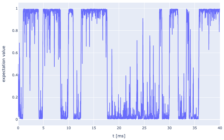
The result can be visualized by providing a list of view operators as follows:
view_ops = {'n':1}
system.plot_transient(view_ops)
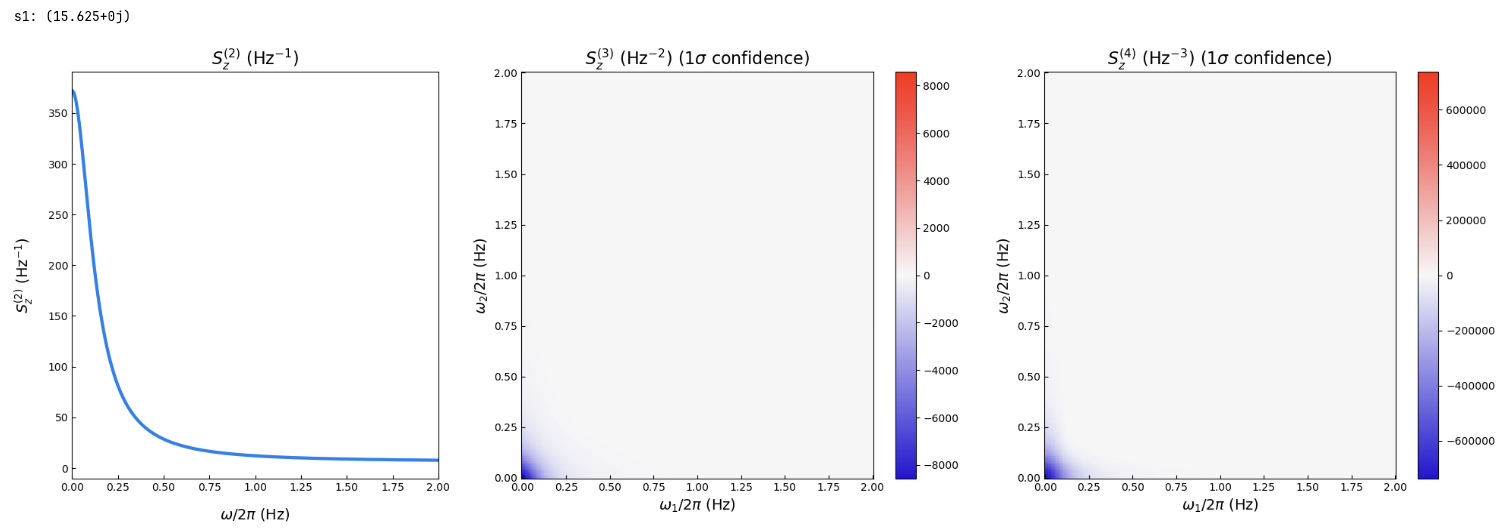
The corresponding quantum polyspectra can be calculated easily via calculate_spectrum function. Refer to the
documentation for the option of this function. For example, here the usage of the GPU can be enabled setting enable_gpu=True.
f_start = 0
f_stop = 2
n_points = 200
fs = np.linspace(f_start, f_stop, n_points)

measure_op = 'n'

spec = system.calculate_spectrum(fs, order_in=[1,2,3,4], measure_op=measure_op)
The polyspectra can be plotted with the plot method:
fig = system.plot()We begin with formulating a model quantum system using standard QuTiP functions.
import quantumcatch as qc
import numpy as np
from qutip import *
The system has to by defined as a function (here set_system) that takes in an array of variable
parameters. We will define the parameters soon, here you simply use the ´params´ dictionary
with you own keys of choice (here gamma_in, gamma_out, and beta). These parameters will
be determined by the fitting routine.
def set_system(params):
    # ------ Operators and Hamiltonian -----
    dot_levels = 2
    a = destroy(dot_levels)
    n = a.dag() * a
    rho_0 = ket2dm(basis(dot_levels, 0)) + ket2dm(basis(dot_levels, 1))
    rho_0 /= np.trace(rho_0)
    H = 0 * n

    # ------ System Parameters ------
    c_measure_strength = {
        'a': params['gamma_out']**0.5,
        'a_d': params['gamma_in']**0.5,
    }

    sc_measure_strength = {
        'n': params['beta']
    }

    c_ops = {
        'a': a,
        'a_d': a.dag(),
    }

    sc_ops =  {
        'n': n,
    }

    e_ops = {
        'n': n,
    }

    system = qc.System(H, rho_0, c_ops, sc_ops, e_ops, c_measure_strength, sc_measure_strength)

    return system, sc_ops, sc_measure_strength
With this parameterize system and the name of our measurement operator, we now create a fit object:
m_op = 'n'
system_fit = qc.FitSystem(set_system, m_op)
Now, we can define the parameters with their starting values and bounds in lmfit fashion.
Assuming that the path leads to spectra calculated and saved with the SignalSnap library,
the fit routine is started with the complete_fit function. Refer to the documentation
for all possible function parameters.
parameter = {'gamma_in':[300, 0, 1e5, True],
             'gamma_out': [700, 0, 1e5, True],
             'beta': [1, 0, 1e12, True],
             'c': [0, -1e12, 1e12, True]}

path = 'example_data/polyspectra_for_fit_example.pkl'
out = system_fit.complete_fit(path, parameter, method='least_squares', xtol=1e-8, ftol=1e-8, fit_modus='resolution_based',
                                                            fit_orders=(1,2,3,4))
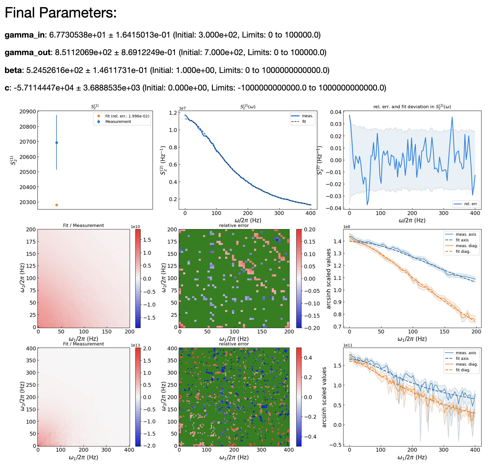
This figure presents a comprehensive set of nine plots designed to evaluate the quality of the fit. The plots are arranged in a 3x3 grid and are interpreted as follows:
-
(0,0): Depicts the first-order spectrum, S1, which is proportional to the mean of the measurement. The experimental S1 trace is displayed in blue, accompanied by its 3σ (three standard deviations) error. The fitted S1 is overlaid in orange.
-
(0,1): Illustrates both the experimental and theoretical power spectra.
-
(0,2): Presents the relative error between the experimental and theoretical power spectra, normalized to the experimental power spectrum, as a blue line. This line can be compared to the 3σ error of the power spectra values.
-
(1,0): Displays the theoretical (upper left triangle) and experimental (lower right triangle) bispectra. This combined representation is facilitated by the symmetry properties of the bispectrum, with the diagonal serving as a symmetry axis.
-
(1,1): Shows the relative error between the experimental and theoretical bispectra, normalized to the experimental bispectrum. A pixel is colored green when the difference between the experimental and theoretical bispectra is less than the 3σ error of the spectral values.
-
(1,2): Features experimental and theoretical bispectral values along the axes (ω1, 0) and the diagonal, accompanied by a 3σ error band.
-
(2,0) to (2,2): These plots mirror the type of plots shown for the bispectrum, but now with the trispectrum.
Each plot provides a unique perspective on the data, collectively offering a robust assessment of the fit's accuracy.
The development of the QunatumCatch package is supported by the working group Spectroscopy of Condensed Matter of the Faculty of Physics and Astronomy at the Ruhr University Bochum.
For the package multiple libraries are used for the numerics and displaying the results:
- Numpy
- Matplotlib
- H5py
- ArrayFire
- Numba
- SciPy
- Tqdm
- Plotly
- Psutil
- Cachetools
- Signalsnap
- Pandas
- Lmfit
- IPyWidgets


