Discover pretrained models for deep learning in MATLAB.
- Image Classification
- Object Detection
- Semantic Segmentation
- Instance Segmentation
- Image Translation
- Pose Estimation
- 3D Reconstruction
- Video Classification
- Text Detection & Recognition
Pretrained image classification networks have already learned to extract powerful and informative features from natural images. Use them as a starting point to learn a new task using transfer learning.
Inputs are RGB images, the output is the predicted label and score:
These networks have been trained on more than a million images and can classify images into 1000 object categories.
Models available in MATLAB:
Note 1: Since R2024a, please use the imagePretrainedNetwork function instead and specify the pretrained model. For example, use the following code to access googlenet:
[net, classes] = imagePretrainedNetwork("googlenet");
| Network | Size (MB) | Classes | Accuracy % | Location |
|---|---|---|---|---|
| googlenet1 | 27 | 1000 | 66.25 | Doc GitHub |
| squeezenet1 | 5.2 | 1000 | 55.16 | Doc |
| alexnet1 | 227 | 1000 | 54.10 | Doc |
| resnet181 | 44 | 1000 | 69.49 | Doc GitHub |
| resnet501 | 96 | 1000 | 74.46 | Doc GitHub |
| resnet1011 | 167 | 1000 | 75.96 | Doc GitHub |
| mobilenetv21 | 13 | 1000 | 70.44 | Doc GitHub |
| vgg161 | 515 | 1000 | 70.29 | Doc |
| vgg191 | 535 | 1000 | 70.42 | Doc |
| inceptionv31 | 89 | 1000 | 77.07 | Doc |
| inceptionresnetv21 | 209 | 1000 | 79.62 | Doc |
| xception1 | 85 | 1000 | 78.20 | Doc |
| darknet191 | 78 | 1000 | 74.00 | Doc |
| darknet531 | 155 | 1000 | 76.46 | Doc |
| densenet2011 | 77 | 1000 | 75.85 | Doc |
| shufflenet1 | 5.4 | 1000 | 63.73 | Doc |
| nasnetmobile1 | 20 | 1000 | 73.41 | Doc |
| nasnetlarge1 | 332 | 1000 | 81.83 | Doc |
| efficientnetb01 | 20 | 1000 | 74.72 | Doc |
| ConvMixer | 7.7 | 10 | - | GitHub |
| Vison Transformer | Large-16 - 1100 Base-16 - 331.4 Small-16 - 84.7 Tiny-16 - 22.2 |
1000 | Large-16 - 85.59 Base-16 - 85.49 Small-16 - 83.73 Tiny-16 - 78.22 |
Doc |
Tips for selecting a model
Pretrained networks have different characteristics that matter when choosing a network to apply to your problem. The most important characteristics are network accuracy, speed, and size. Choosing a network is generally a tradeoff between these characteristics. The following figure highlights these tradeoffs:
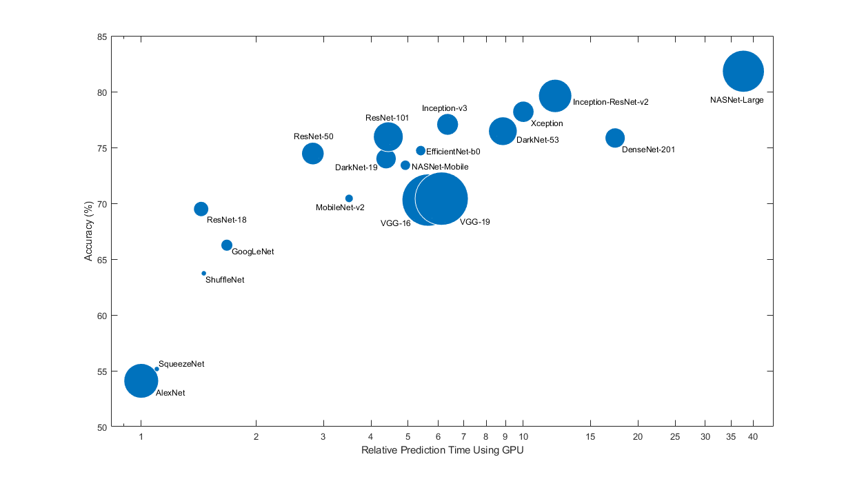 Figure. Comparing image classification model accuracy, speed and size.
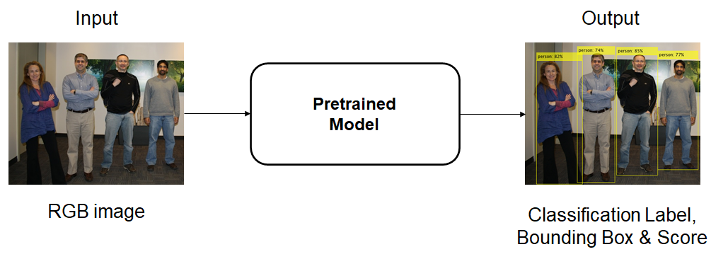
Object detection is a computer vision technique used for locating instances of objects in images or videos. When humans look at images or video, we can recognize and locate objects of interest within a matter of moments. The goal of object detection is to replicate this intelligence using a computer.
Inputs are RGB images, the output is the predicted label, bounding box and score:
These networks have been trained to detect 80 objects classes from the COCO dataset. These models are suitable for training a custom object detector using transfer learning.
| Network | Network variants | Size (MB) | Mean Average Precision (mAP) | Object Classes | Location |
|---|---|---|---|---|---|
| EfficientDet-D0 | efficientnet | 15.9 | 33.7 | 80 | GitHub |
| YOLO v8 | yolo8n yolo8s yolo8m yolo8l yolo8x |
10.7 37.2 85.4 143.3 222.7 |
37.3 44.9 50.2 52.9 53.9 |
80 | GitHub |
| YOLOX | YoloX-s YoloX-m YoloX-l |
32 90.2 192.9 |
39.8 45.9 48.6 |
80 | Doc GitHub |
| YOLO v4 | yolov4-coco yolov4-tiny-coco |
229 21.5 |
44.2 19.7 |
80 | Doc GitHub |
| YOLO v3 | darknet53-coco tiny-yolov3-coco |
220.4 31.5 |
34.4 9.3 |
80 | Doc |
| YOLO v2 | darknet19-COCO tiny-yolo_v2-coco |
181 40 |
28.7 10.5 |
80 | Doc GitHub |
Tips for selecting a model
Pretrained object detectors have different characteristics that matter when choosing a network to apply to your problem. The most important characteristics are mean average precision (mAP), speed, and size. Choosing a network is generally a tradeoff between these characteristics.
Application Specific Object Detectors
These networks have been trained to detect specific objects for a given application.
| Network | Application | Size (MB) | Location | Example Output |
|---|---|---|---|---|
| Spatial-CNN | Lane detection | 74 | GitHub | 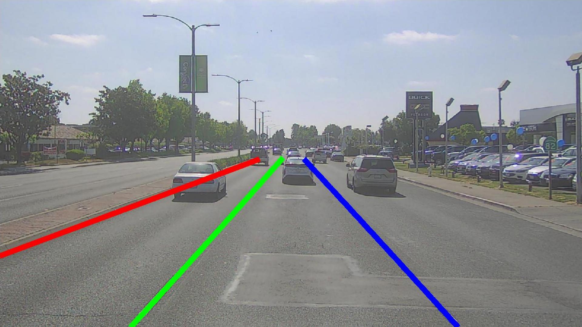 |
| RESA | Road Boundary detection | 95 | GitHub | 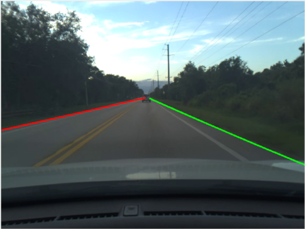 |
| Single Shot Detector (SSD) | Vehicle detection | 44 | Doc | 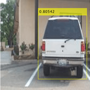 |
| Faster R-CNN | Vehicle detection | 118 | Doc | 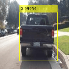 |
Segmentation is essential for image analysis tasks. Semantic segmentation describes the process of associating each pixel of an image with a class label, (such as flower, person, road, sky, ocean, or car).
Inputs are RGB images, outputs are pixel classifications (semantic maps).
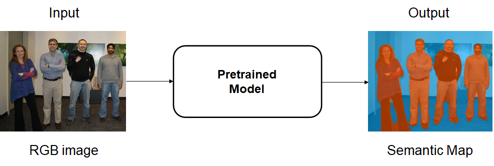
This network has been trained to detect 20 objects classes from the PASCAL VOC dataset:
| Network | Size (MB) | Mean Accuracy | Object Classes | Location |
|---|---|---|---|---|
| DeepLabv3+ | 209 | 0.87 | 20 | GitHub |
Zero-shot image segmentation model:
| Network | Size (MB) | Example Location |
|---|---|---|
| segmentAnythingModel | 358 | Doc |
Application Specific Semantic Segmentation Models
| Network | Application | Size (MB) | Location | Example Output |
|---|---|---|---|---|
| U-net | Raw Camera Processing | 31 | Doc | 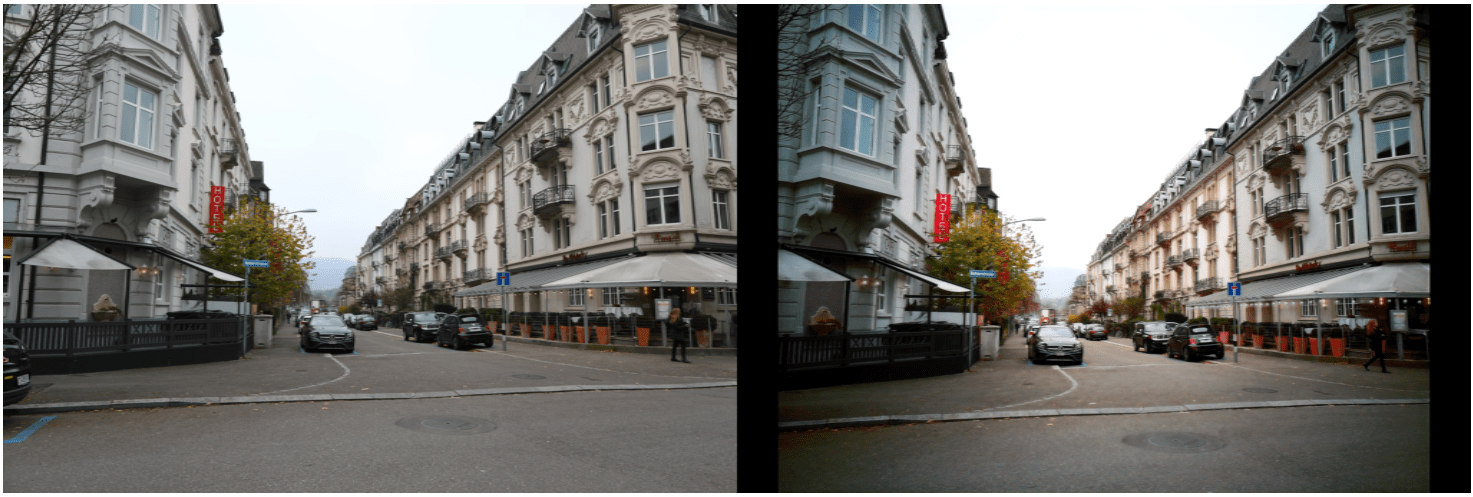 |
| 3-D U-net | Brain Tumor Segmentation | 56.2 | Doc | 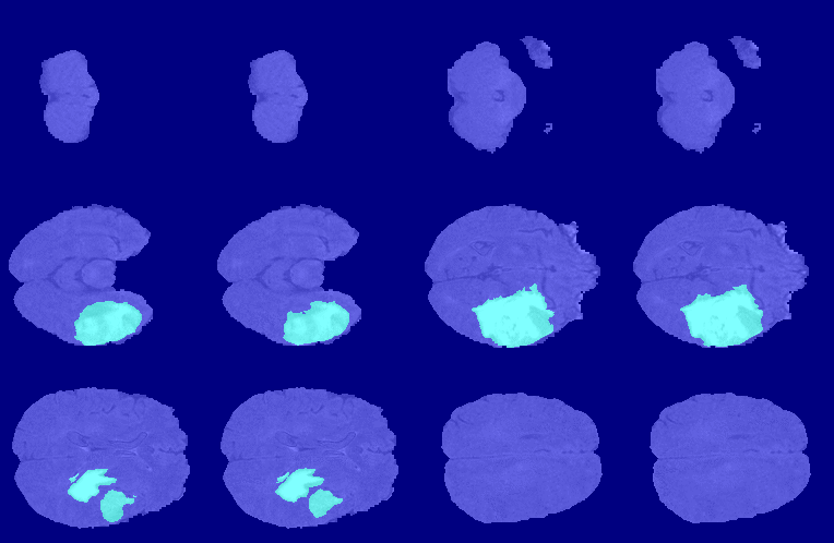 |
| AdaptSeg (GAN) | Model tuning using 3-D simulation data | 54.4 | Doc | 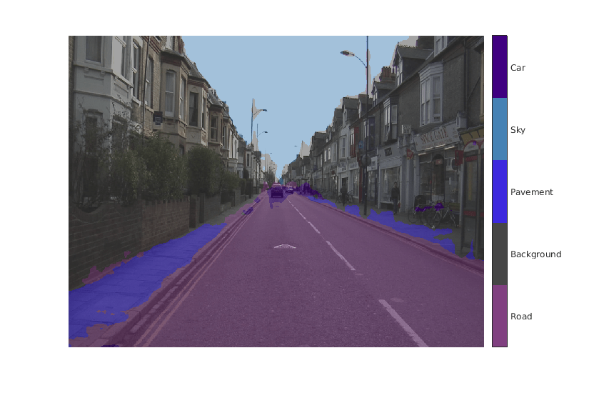 |
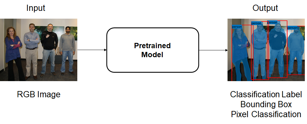
Instance segmentation is an enhanced type of object detection that generates a segmentation map for each detected instance of an object. Instance segmentation treats individual objects as distinct entities, regardless of the class of the objects. In contrast, semantic segmentation considers all objects of the same class as belonging to a single entity.
Inputs are RGB images, outputs are pixel classifications (semantic maps), bounding boxes and classification labels.
| Network | Object Classes | Location |
|---|---|---|
| Mask R-CNN | 80 | Doc Github |
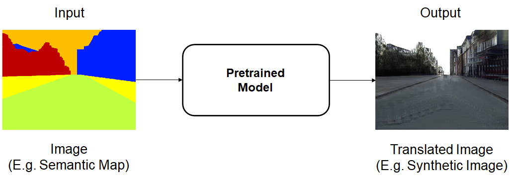
Image translation is the task of transferring styles and characteristics from one image domain to another. This technique can be extended to other image-to-image learning operations, such as image enhancement, image colorization, defect generation, and medical image analysis.
Inputs are images, outputs are translated RGB images. This example workflow shows how a semantic segmentation map input translates to a synthetic image via a pretrained model (Pix2PixHD):
| Network | Application | Size (MB) | Location | Example Output |
|---|---|---|---|---|
| Pix2PixHD(CGAN) | Synthetic Image Translation | 648 | Doc | 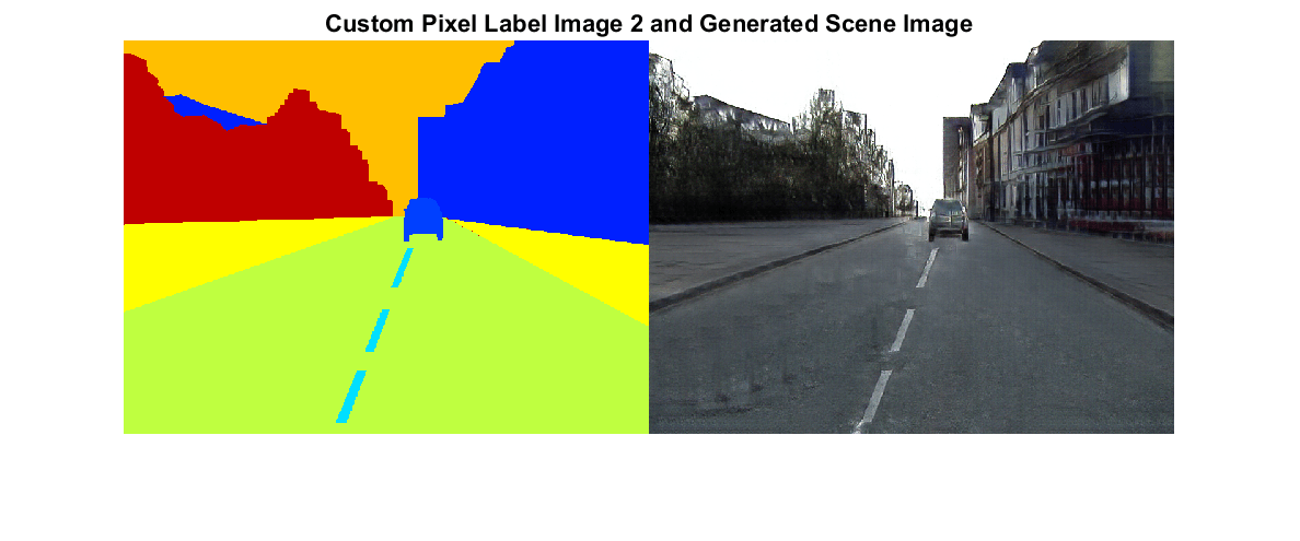 |
| UNIT (GAN) | Day-to-Dusk Dusk-to-Day Image Translation | 72.5 | Doc | 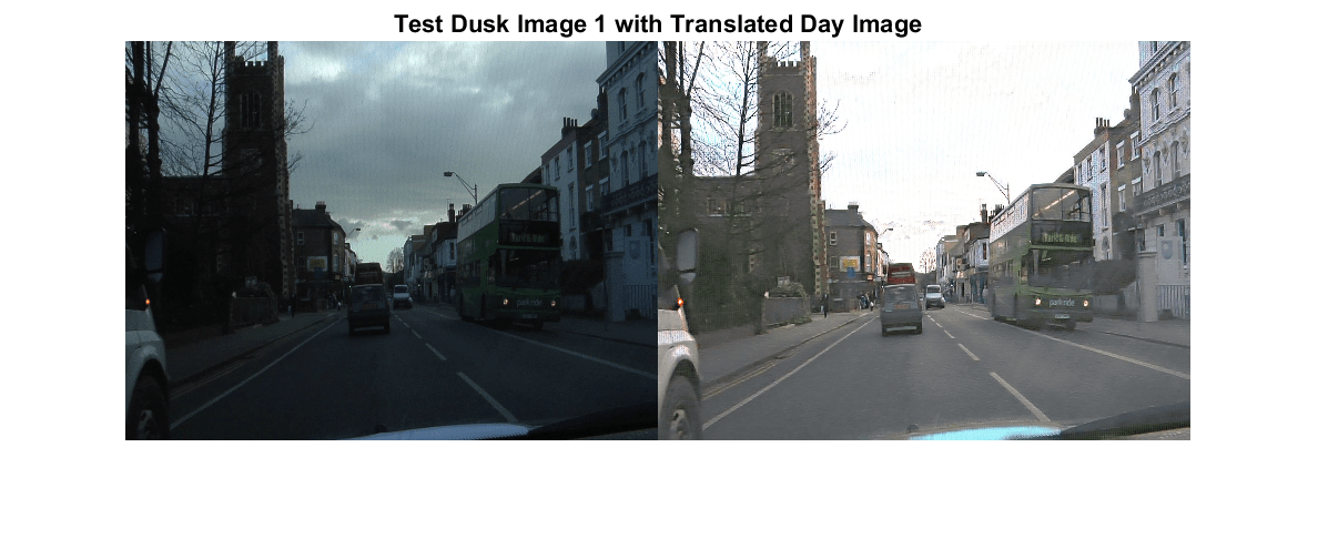 |
| UNIT (GAN) | Medical Image Denoising | 72.4 | Doc | 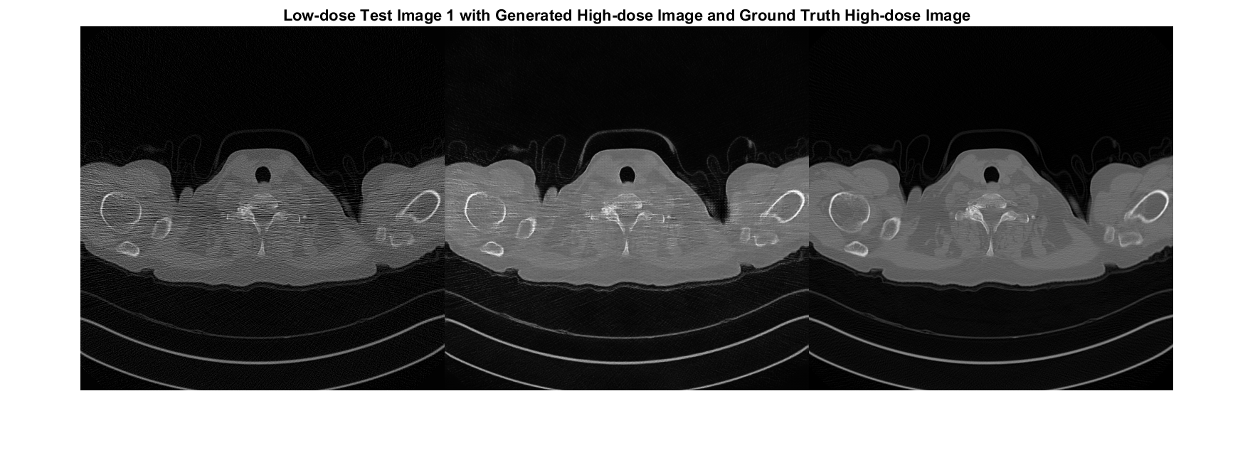 |
| CycleGAN | Medical Image Denoising | 75.3 | Doc | 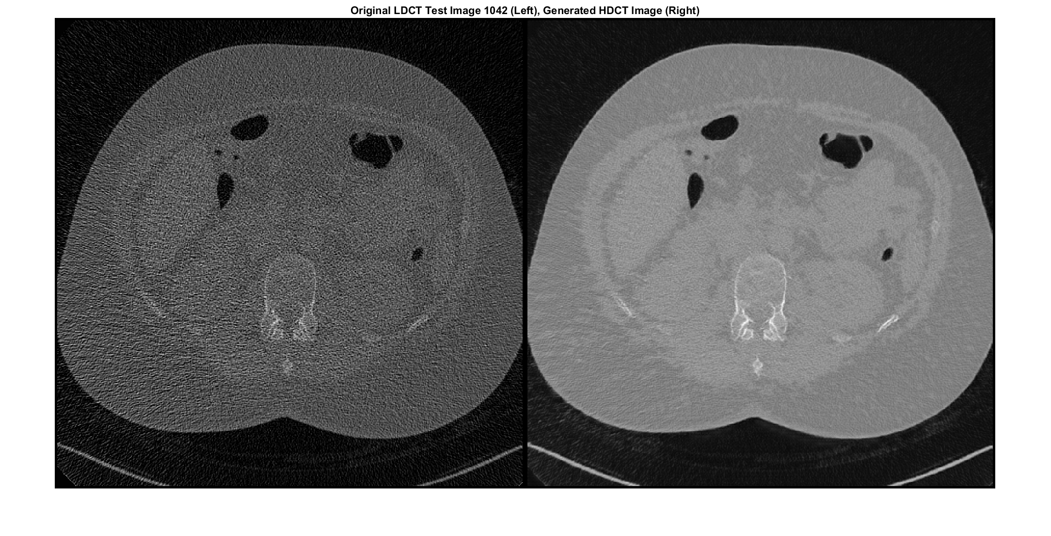 |
| VDSR | Super Resolution (estimate a high-resolution image from a low-resolution image) | 2.4 | Doc | 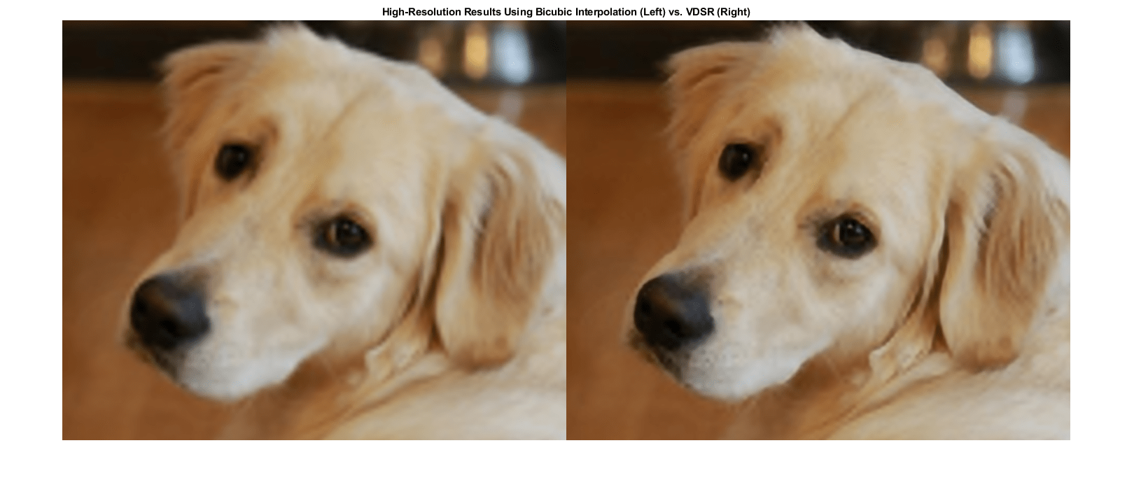 |
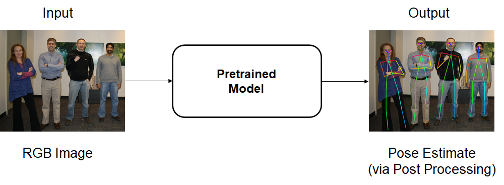
Pose estimation is a computer vision technique for localizing the position and orientation of an object using a fixed set of keypoints.
All inputs are RGB images, outputs are heatmaps and part affinity fields (PAFs) which via post processing perform pose estimation.
| Network | Backbone Networks | Size (MB) | Location |
|---|---|---|---|
| OpenPose | vgg19 | 14 | Doc |
| HR Net | human-full-body-w32 human-full-body-w48 |
106.9 237.7 |
Doc |
3D reconstruction is the process of capturing the shape and appearance of real objects.
| Network | Size (MB) | Location | Example Output |
|---|---|---|---|
| NeRF | 3.78 | GitHub |  |
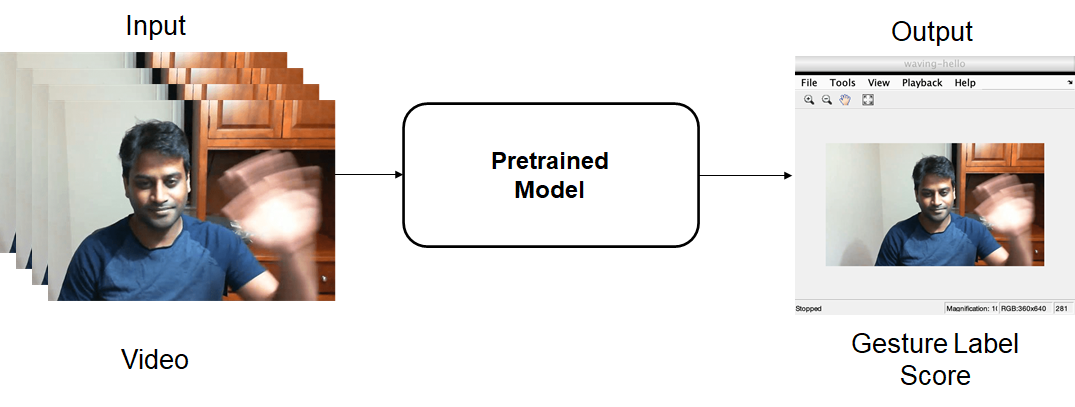
Video classification is a computer vision technique for classifying the action or content in a sequence of video frames.
All inputs are Videos only or Video with Optical Flow data, outputs are gesture classifications and scores.
| Network | Inputs | Size(MB) | Classifications (Human Actions) | Description | Location |
|---|---|---|---|---|---|
| SlowFast | Video | 124 | 400 | Faster convergence than Inflated-3D | Doc |
| R(2+1)D | Video | 112 | 400 | Faster convergence than Inflated-3D | Doc |
| Inflated-3D | Video & Optical Flow data | 91 | 400 | Accuracy of the classifier improves when combining optical flow and RGB data. | Doc |
Text detection is a computer vision technique used for locating instances of text within in images.
Inputs are RGB images, outputs are bounding boxes that identify regions of text.
| Network | Application | Size (MB) | Location |
|---|---|---|---|
| CRAFT | Trained to detect English, Korean, Italian, French, Arabic, German and Bangla (Indian). | 3.8 | Doc GitHub |
Application Specific Text Detectors
| Network | Application | Size (MB) | Location | Example Output |
|---|---|---|---|---|
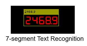
| Seven Segment Digit Recognition | Seven segment digit recognition using deep learning and OCR. This is helpful in industrial automation applications where digital displays are often surrounded with complex background. | 3.8 | Doc GitHub |
 |
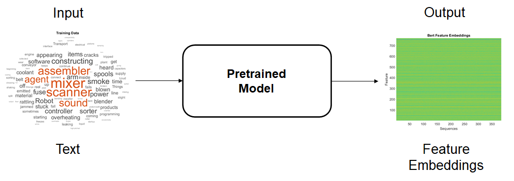
Transformer pretained models have already learned to extract powerful and informative features features from text. Use them as a starting point to learn a new task using transfer learning.
Inputs are sequences of text, outputs are text feature embeddings.
| Network | Applications | Size (MB) | Location |
|---|---|---|---|
| BERT | Feature Extraction (Sentence and Word embedding), Text Classification, Token Classification, Masked Language Modeling, Question Answering | 390 | GitHub Doc |
| all-MiniLM-L6-v2 | Document Embedding, Clustering, Information Retrieval | 80 | Doc |
| all-MiniLM-L12-v2 | Document Embedding, Clustering, Information Retrieval | 120 | Doc |
Application Specific Transformers
| Network | Application | Size (MB) | Location | Output Example |
|---|---|---|---|---|
| FinBERT | The FinBERT model is a BERT model for financial sentiment analysis | 388 | GitHub | 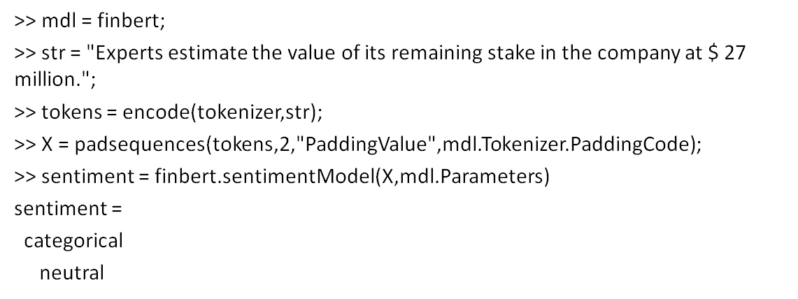 |
| GPT-2 | The GPT-2 model is a decoder model used for text summarization. | 1.2GB | GitHub |  |
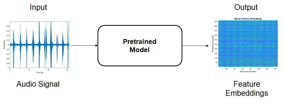
Audio embedding pretrained models have already learned to extract powerful and informative features from audio signals. Use them as a starting point to learn a new task using transfer learning.
Inputs are audio signals, outputs are audio feature embeddings.
Note 2: Since R2024a, please use the audioPretrainedNetwork function instead and specify the pretrained model. For example, use the following code to access VGGish:
net = audioPretrainedNetwork("vggish");
| Network | Application | Size (MB) | Location |
|---|---|---|---|
| VGGish2 | Feature Embeddings | 257 | Doc |
| OpenL32 | Feature Embeddings | 200 | Doc |
| Network | Application | Size (MB) | Output Classes | Location | Output Example |
|---|---|---|---|---|---|
| vadnet2 | Voice Activity Detection (regression) | 0.427 | - | Doc | 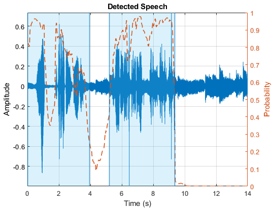 |
| YAMNet2 | Sound Classification | 13.5 | 521 | Doc | 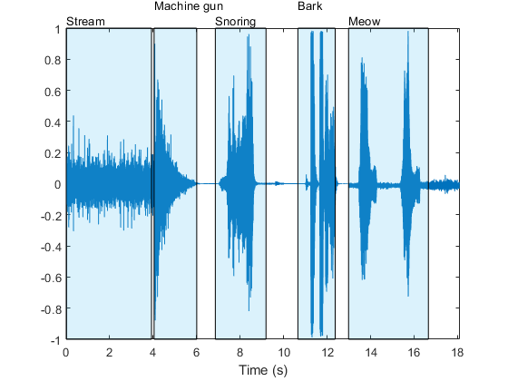 |
| CREPE2 | Pitch Estimation (regression) | 132 | - | Doc | 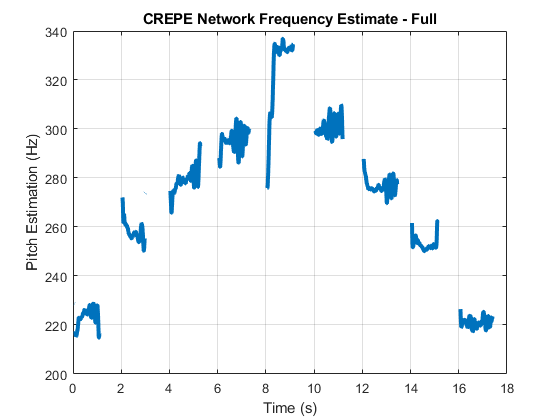 |
Speech-to-text models provide a fast, efficient method to convert spoken language into written text, enhancing accessibility for individuals with disabilities, enabling downstream tasks like text summarization and sentiment analysis, and streamlining documentation processes. As a key element of human-machine interfaces, including personal assistants, it allows for natural and intuitive interactions, enabling machines to understand and execute spoken commands, improving usability and broadening inclusivity across various applications.
Inputs are audio signals, outputs is text.
| Network | Application | Size (MB) | Word Error Rate (WER) | Location |
|---|---|---|---|---|
| wav2vec | Speech to Text | 236 | 3.2 | GitHub |
| deepspeech | Speech to Text | 167 | 5.97 | GitHub |
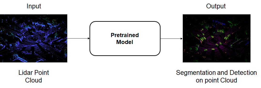
Point cloud data is acquired by a variety of sensors, such as lidar, radar, and depth cameras. Training robust classifiers with point cloud data is challenging because of the sparsity of data per object, object occlusions, and sensor noise. Deep learning techniques have been shown to address many of these challenges by learning robust feature representations directly from point cloud data.
Inputs are Lidar Point Clouds converted to five-channels, outputs are segmentation, classification or object detection results overlayed on point clouds.
| Network | Application | Size (MB) | Object Classes | Location |
|---|---|---|---|---|
| PointNet | Classification | 5 | 14 | Doc |
| PointNet++ | Segmentation | 3 | 8 | Doc |
| PointSeg | Segmentation | 14 | 3 | Doc |
| SqueezeSegV2 | Segmentation | 5 | 12 | Doc |
| SalsaNext | Segmentation | 20.9 | 13 | GitHub |
| PointPillars | Object Detection | 8 | 3 | Doc |
| Complex YOLO v4 | Object Detection | 233 (complex-yolov4) 21 (tiny-complex-yolov4) |
3 | GitHub |
Manipulator motion planning is a technique used to plan a trajectory for a robotic arm from a start position to a goal position in an obstacle environment.
Pretrained deep learning models have learned to plan such trajectories for repetitive tasks such as picking and placing of objects, leading to speed ups over traditional algorithms.
Inputs are start configuration, goal configuration and obstacle environment encoding for the robot, outputs are intermediate trajectory guesses.
| Network | Application | Size (MB) | Location |
|---|---|---|---|
| Deep-Learning-Based CHOMP (DLCHOMP) | Trajectory Prediction | 25 | Doc GitHub |
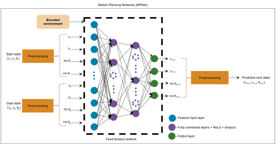
Motion Planning Networks (MPNet) is a deep-learning-based approach for finding optimal paths between a start point and goal point in motion planning problems. MPNet is a deep neural network that can be trained on multiple environments to learn optimal paths between various states in the environments. The MPNet uses this prior knowledge to,
- Generate informed samples between two states in an unknown test environment. These samples can be used with sampling-based motion planners such as optimal rapidly-exploring random trees (RRT*) for path planning.
- Compute collision-free path between two states in an unknown test environment. MPNet based path planner is more efficient than the classical path planners such as the RRT*.
To know more please visit Get Started with Motion Planning Networks
| Network | Application | Size (MB) | Location |
|---|---|---|---|
| mazeMapTrainedMPNET | Path Planning | 0.23 | Doc |
If you'd like to request MATLAB support for additional pretrained models, please create an issue from this repo.
Alternatively send the request through to:
Jianghao Wang
Deep Learning Product Manager
jianghaw@mathworks.com
Copyright 2024, The MathWorks, Inc.

