readeba

{readeba} helps you download and import data on enterprise agreement settlements in Australia from the Fair Work Commission.

Installation

You can install {readeba} from GitHub with:

# install.packages("devtools")
devtools::install_github("MattCowgill/readeba")

Examples!

The package has one function: read_fwc(), which downloads and imports a tidy tibble containing the FWC EBA data

library(readeba)
library(dplyr)
#> 
#> Attaching package: 'dplyr'
#> The following objects are masked from 'package:stats':
#> 
#>     filter, lag
#> The following objects are masked from 'package:base':
#> 
#>     intersect, setdiff, setequal, union
library(ggplot2)
library(tidyr)

fwc <- read_fwc()

fwc 
#> # A tibble: 1,194 × 4
#>    date       indicator               union  value
#>    <date>     <chr>                   <chr>  <dbl>
#>  1 2022-07-15 Employees covered (No.) Total  19132
#>  2 2022-07-29 Employees covered (No.) Total  20038
#>  3 2022-08-12 Employees covered (No.) Total  15331
#>  4 2022-08-26 Employees covered (No.) Total  10065
#>  5 2022-09-09 Employees covered (No.) Total  26461
#>  6 2022-09-23 Employees covered (No.) Total  16551
#>  7 2022-10-07 Employees covered (No.) Total  21586
#>  8 2022-10-21 Employees covered (No.) Total  16503
#>  9 2022-11-04 Employees covered (No.) Total 100074
#> 10 2022-11-18 Employees covered (No.) Total  24113
#> # ℹ 1,184 more rows

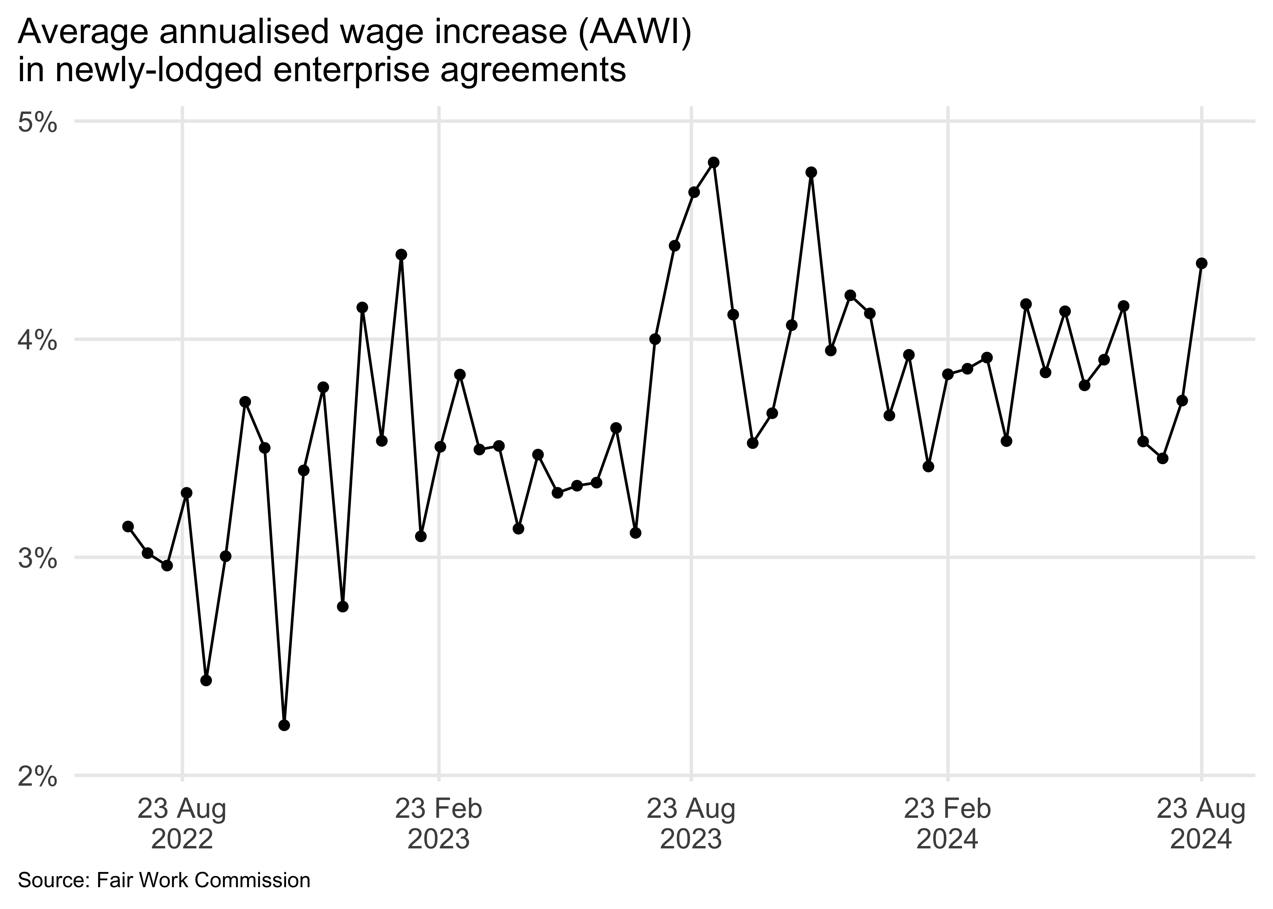
It’s straightforward to visualise!

my_theme <- theme_minimal(base_size = 14) +
  theme(panel.grid.minor = element_blank(),
        axis.title = element_blank(),
        plot.caption.position = "plot",
        plot.title.position = "plot",
        plot.caption = element_text(size = rel(0.6), hjust = 0),
        legend.position = "bottom",
        legend.direction = "horizontal")


fwc |> 
  filter(union == "Total",
         indicator == "AAWI (%)") |> 
  ggplot(aes(x = date, y = value)) +
  geom_point() +
  geom_line() +
  scale_x_date(date_labels = "%d %b\n%Y",
               breaks = seq(max(fwc$date),
                            min(fwc$date),
                            "-6 months")) +
  scale_y_continuous(labels = \(x) paste0(x, "%"),
                     expand = expansion(0.1)) +
  my_theme +
  labs(subtitle = "Average annualised wage increase (AAWI)\nin newly-lodged enterprise agreements",
       caption = "Source: Fair Work Commission")

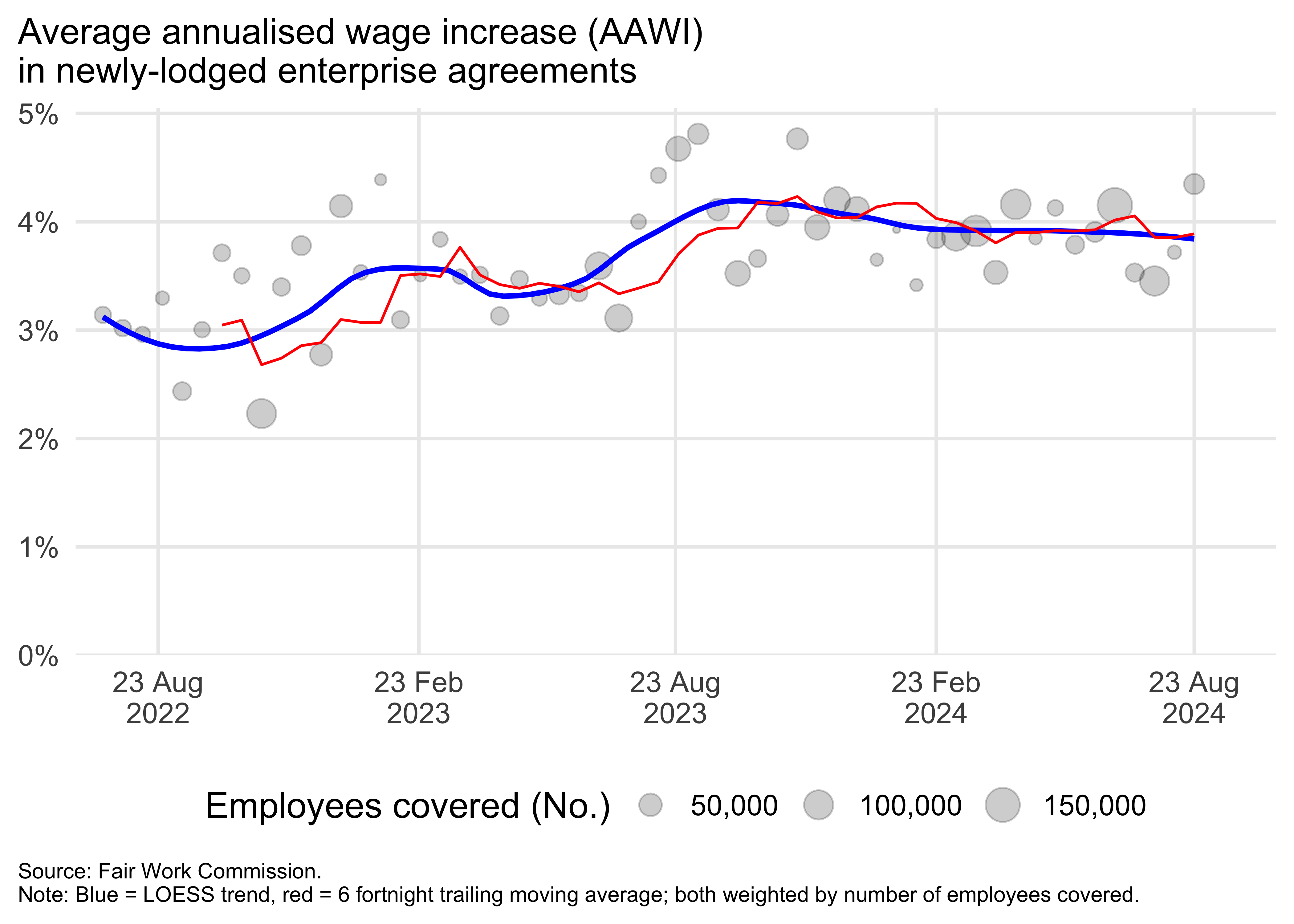
Add a couple of different trend lines:

fwc |> 
  filter(union == "Total") |> 
  pivot_wider(names_from = indicator) |> 
  ggplot(aes(x = date, 
             y = `AAWI (%)`,
             weight = `Employees covered (No.)` )) +
  geom_point(aes(size = `Employees covered (No.)`),
             alpha = 0.2) +
  geom_smooth(method = "loess",
              formula = y ~ x,
              se = FALSE,
              colour = "blue",
              span = 0.5) +
  geom_line(aes(y = slider::slide2_dbl(.x = `AAWI (%)`,
                                       .y = `Employees covered (No.)`,
                                       .f = \(x, y) weighted.mean(x, y),
                                       .before = 6L,
                                       .complete = TRUE)),
            na.rm = TRUE,
            colour = "red") +
  scale_x_date(breaks = seq(max(fwc$date), 
                            min(fwc$date), 
                            by = "-6 months"),
               date_labels = "%d %b\n%Y",
               expand = expansion(c(0.025, 0.075))) +
  scale_y_continuous(labels = \(x) paste0(x, "%"),
                     breaks = seq(0, 100, 1),
                     limits = \(x) c(min(0, x[1]), x[2]),
                     expand = expansion(c(0, 0.05))) +
  scale_size_continuous(labels = scales::comma) +
  my_theme +
  labs(subtitle = "Average annualised wage increase (AAWI)\nin newly-lodged enterprise agreements ",
       caption = "Source: Fair Work Commission.\nNote: Blue = LOESS trend, red = 6 fortnight trailing moving average; both weighted by number of employees covered.")