{readjsa} streamlines the process of getting data from Jobs and Skills Australia into R.
Note that this package is marked experimental. The code is stable, but brittle. Any changes by JSA to its data and how it’s distributed are likely to break the functionality of the package, at least temporarily.
You can install the development version of readjsa from GitHub with :
# install.packages("devtools")
devtools::install_github("MattCowgill/readjsa")At the moment, {readjsa} can be used to get data from the Recruitment
Experience & Outlook Survey (REOS), the Internet Vacancy Index (IVI),
and Small Area Labour Markets (SALM). The functions for doing so are
read_reos, read_ivi, and read_salm respectively - see below for
more.
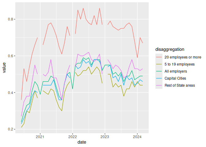
It’s straightforward to get data from the JSA REOS:
library(readjsa)
library(ggplot2)
library(dplyr)
#>
#> Attaching package: 'dplyr'
#> The following objects are masked from 'package:stats':
#>
#>     filter, lag
#> The following objects are masked from 'package:base':
#>
#>     intersect, setdiff, setequal, union

reos <- read_reos(tables = "all")

reos |>
  filter(
    series == "Recruitment rate",
    frequency == "Monthly"
  ) |>
  ggplot(aes(x = date, y = value, col = disaggregation)) +
geom_line()There are several different tables in the IVI data, at different levels
of aggregation. See ?read_ivi(). In the example below, we’re
visualising total job vacancies at the state level.
ivi_states <- read_ivi("2dig_states")

ivi_states |>
  filter(
    level == 1,
    state != "AUST"
  ) |>
  ggplot(aes(x = date, y = value, col = series_type)) +
  geom_line() +
  facet_wrap(~state,
    scales = "free_y",
    nrow = 2
  ) +
  theme(
    legend.position = "bottom",
    legend.direction = "horizontal"
)There are three SALM tables (total labour force in persons, total
unemployment in persons, and unemployment rate) available by either
Statistical Area Level 2 (SA2) and Local Government Area (LGA) levels.
See ?read_salm() for more information, and the JSA
website
for methodology and usage recommendations.
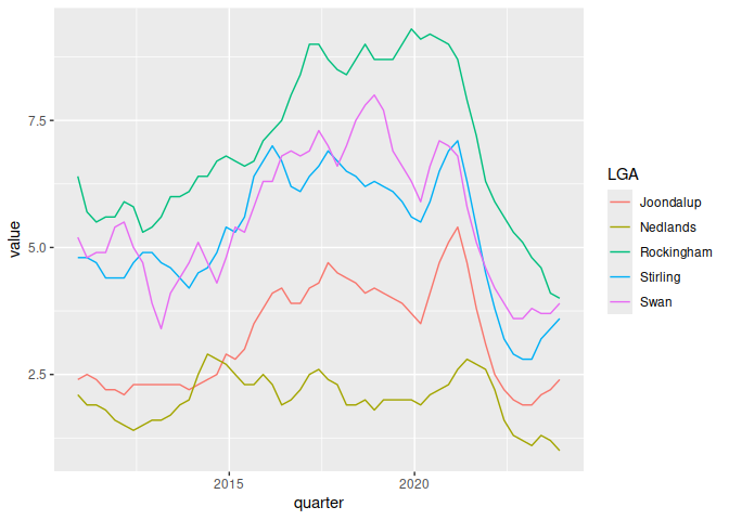
In this example, we visualise smoothed estimates of unemployment rates across five LGAs in Perth since 2010.
salm_LGA <- read_salm("unemp_rate")
perth_LGAs <- c("Stirling", "Joondalup", "Nedlands", "Swan", "Rockingham")

salm_LGA |>
  rename(LGA = local_government_area_lga_2023_asgs) |>
  filter(
    LGA %in% perth_LGAs
  ) |>
  ggplot(aes(
    x = quarter,
    y = value,
    col = LGA
  )) +
  geom_line()

