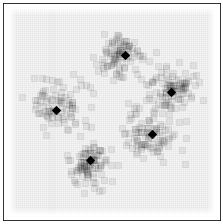
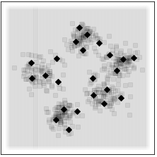
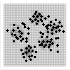
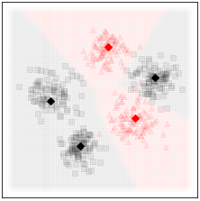
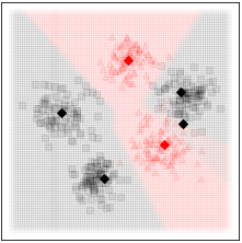
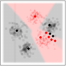
A general-purpose learning model designed to meet the needs of applications in which computational resources are limited, and robustness and interpretability are prioritized.
Constitutes an online prototype-based learning algorithm based on annealing optimization that is formulated as an recursive gradient-free stochastic approximation algorithm.
Can be viewed as an interpretable and progressively growing competitive-learning neural network model.
Applications include online unsupervised and supervised learning [1], regression, reinforcement learning [2], adaptive graph partitioning [3], and swarm leader detection.
Christos N. Mavridis, Ph.D.
Department of Electrical and Computer Engineering,
University of Maryland
https://mavridischristos.github.io/
mavridis (at) umd.edu
The observed data are represented by a random variable
Given a similarity measure (which can be any Bregman divergence, e.g., squared Euclidean distance, Kullback-Leibler divergence, etc.)
For supervised learning, e.g., classification and regression, each codevector
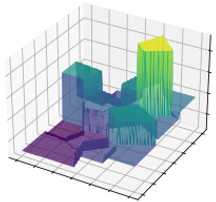
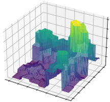
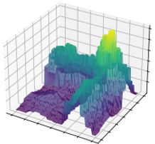
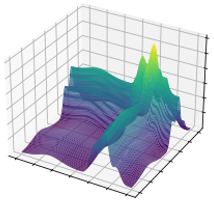
Piecewise-constant approximation (partition) of the input space
$S$ .
To construct a learning algorithm that progressively increases the number
of codevectors
First we need to adopt a probabilistic approach, and a discrete random variable
Then we constraint its distribution by formulating the multi-objective optimization:
This is now a problem of finding the locations
The Lagrange multiplier
$T\in[0,1]$ is called the temperature parameter
and controls the trade-off between
Reducing the values of
$T$ results in a bifurcation phenomenon that increases$M$ and describes an annealing process [1, 2].
The above sequence of optimization problems is solved for decreasing values of T using a
Recursive gradient-free stochastic approximation algorithm.
The annealing nature of the algorithm contributes to avoiding poor local minima, offers robustness with respect to the initial conditions, and provides a means to progressively increase the complexity of the learning model through an intuitive bifurcation phenomenon.
The ODA architecture is coded in the ODA class inside OnlineDeterministicAnnealing/oda.py:
from oda import ODA
Regarding the data format, they need to be a list of (n) lists of (m=1) d-vectors (np.arrays):
train_data = [[np.array], [np.array], [np.array], ...]
The simplest way to train ODA on a dataset is:
clf = ODA(train_data=train_data,train_labels=train_labels)
clf.fit(test_data=test_data,test_labels=test_labels)
Notice that a dataset is not required, and one can train ODA using observations one at a time as follows:
tl = len(clf.timeline)
# Stop in the next converged configuration
while len(clf.timeline)==tl and not clf.trained:
    train_datum, train_label = system.observe()
    clf.train(train_datum,train_label,test_data=test_data,test_labels=test_labels)
For classification, the labels need to be a list of (n) labels, preferably integer numbers (for numba.jit)
train_labels = [ int, int , int, ...]
For clustering replace:
train_labels = [0 for i in range(len(train_labels))]
For regression (piece-wise constant function approximation) replace:
train_labels = [ np.array, np.array , np.array, ...]
clf = ODA(train_data=train_data,train_labels=train_labels,regression=True)
prediction = clf.predict(test_datum)
error = clf.score(test_data, test_labels)
Bregman Divergence:
# Values in {'phi_Eucl', 'phi_KL'} (Squared Euclidean distance, KL divergence)
Bregman_phi = ['phi_Eucl']
Minimum Termperature
Tmin = [1e-4]
Limit in node's children. After that stop growing
Kmax = [50]
Desired training error
error_threshold = [0.0]
# Stop when reached 'error_threshold_count' times
error_threshold_count = [2]
# Make sure keepscore > 2
ODA vs Soft-Clustering vs LVQ
# Values in {0,1,2,3}
# 0:ODA update
# 1:ODA until Kmax. Then switch to 2:soft clustering with no perturbation/merging
# 2:soft clustering with no perturbation/merging
# 3: LVQ update (hard-clustering) with no perturbation/merging
lvq=[0]
Verbose
# Values in {0,1,2,3}
# 0: don't compute or show score
# 1: compute and show score only on tree node splits
# 2: compute score after every SA convergence and use it as a stopping criterion
# 3: compute and show score after every SA convergence and use it as a stopping criterion
keepscore = 3
The history of all the intermediate models trained is stored in:
clf.myY, clf.myYlabels, clf.myK, clf.myTreeK, clf.myT, clf.myLoops, clf.myTime, clf.myTrainError, clf.myTestError
For multiple resolutions every parameter becomes a list of m parameters. Example for m=2:
Tmax = [0.9, 0.09]
Tmin = [0.01, 0.0001]
The training data should look like this:
train_data = [[np.array, np.array, ...], [np.array, np.array, ...], [np.array, np.array, ...], ...]
If you use this work in an academic context, please cite the following:
[1] Christos N. Mavridis and John S. Baras, "Online Deterministic Annealing for Classification and Clustering", IEEE TCNS, 2022.
@article{mavridis2022online,
      title={Online Deterministic Annealing for Classification and Clustering},
      author={Mavridis, Christos N. and Baras, John S.},
      journal={IEEE Transactions on Neural Networks and Learning Systems},
      year={2022},
      volume={},
      number={},
      pages={1-10},
      doi={10.1109/TNNLS.2021.3138676}
      }
Other references:
[2] Christos N. Mavridis and John S. Baras, "Annealing Optimization for Progressive Learning with Stochastic Approximation", arXiv:2209.02826.
[3] Christos N. Mavridis and John S. Baras, "Maximum-Entropy Input Estimation for Gaussian Processes in Reinforcement Learning", CDC, 2021.
[4] Christos N. Mavridis and John S. Baras, "Progressive Graph Partitioning Based on Information Diffusion", CDC, 2021.
