MaxtBIT/Summary-of-Codes-for-HSI-Reconstruction

A summary of CASSI reconstruction algorithms, including performance, complexity, paper links and codes.

Summary of Reconstruction Algorithms for CASSI

Coded Aperture Snapshot Spectral Imaging(CASSI) is a cutting-edge technology of spectral imaging. The reconstruction algorithms of CASSI, which are devoted to solve the inverse imaging problem, determine the quality and efficiency of imaging. Given the sensing matrix A and the 2D CASSI measurement y, estimating the underlying image x is the fundamental task of reconstruction.

In the site, the mainstream algorithms are summarized according to different datasets. They are quantitatively evaluated in terms of performance and complexity. The distortion, including peak signal-to-noise ratio (PSNR), structural similarity (SSIM) and spectral angle mapping (SAM), are usually utilized to evaluate the performance of the algorithms. The functions for calculation are provided in cal_distortion.py. Meanwhile, parameters(Params) counts and floating-point operations(FLOPs) counts are utilized to measure the model complexity. The functions for calculation are provided in cal_complexity.py.

Environment

Python 3.6.2
CUDA 10.0
Torch 1.7.0
SciPy 1.5.4
CuPy 9.6.0
OpenCV 4.5.4
NumPy 1.19.5

Usage

1. Download this repository via git or download the ZIP file manually.

git clone https://github.com/MaxtBIT/Summary-of-Codes-for-HSI-Reconstruction.git

2. Create the environment and ensure the version.
3. Select a method in cal_complexity.py. Then, run this file to get Params and FLOPs.
4. The function to calculate distortion can be checked in cal_distortion.py.

ICVL Dataset

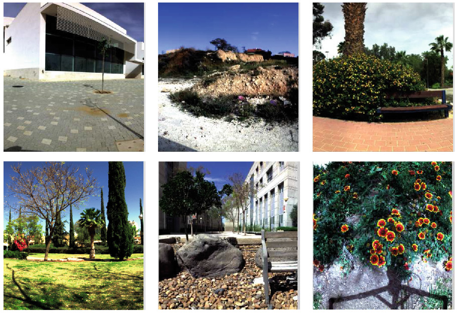
The spectral images in the ICVL Dataset are acquired using a Specim PS Kappa DX4 spectral camera and a rotary stage for spatial scanning. The spectral range is from 400nm to 700nm, which is divided into 31 spectral bands with approximate 10nm bandwidth for each band. There are 201 spectral images in ICVL Dataset. To avoid over-fitting, 31 spectral images with similar backgrounds and 20 spectral images with similar contents are excluded. Then, 100 spectral images are randomly selected for training, and 50 spectral images are used for testing. The specific splitting can be checked in ./data/ICVL_Dataset.txt.

Click here to download ICVL Dataset.

1.Configurations

To derive the simulative measurement, first, the coded aperture pattern is constructed by following random matrix in Bernoulli distributions with p = 0.5. Then, the coded aperture pattern is upsampled and shifted into the sensing matrix. Afterwards, a Hadamard product is made between a spectral image and the sensing matrix to simulate degradation. Finally, the degraded image is projected into a 2D image along the spectral dimension, i.e., the measurement. In training, the simulative measurement and the corresponding spectral image are paired to supervise the parameters updating. In testing, only the central areas with 256 * 256 * 31 or 512 * 512 * 31 are compared to evaluate the performance.

2.Results

Comparison of performance and complexity on ICVL Dataset (The ' indicates that the maximum pixel value used in the calculation of PSNR is 1.0)

Year	Method	Performance					Complexity
		Size	PSNR	SSIM	Source	Code Link	Params(M)	FLOPs(GMac)
2021	DRAN	256*256	38.900'	0.980	Original Paper	Private	/	/
2021	DEIL	512*512	36.571	0.995	Original Paper	Private	/	/
2021	DTLP	256*256	34.530	0.977	Original Paper	PyTorch TensorFlow	3.20	185.47
2020	DNU	512*512	34.270	0.991	Original Paper	PyTorch	4.21	1104.96
		512*512	33.784	0.991	Reproduced Paper
2019	DSSP	256*256	39.670'	0.979	Reproduced Paper	TensorFlow	0.334	22.42
		512*512	34.130	0.992	Original Paper			89.68
2019	HyperR- econNet	256*256	38.430'	0.972	Reproduced Paper	PyTorch Caffe	3.86	393.12
		512*512	32.363	0.986	Original Paper			1572.48
2019	λ-Net	256*256	29.006	0.946	Reproduced Paper	TensorFlow	58.26	44.82
		512*512	28.850	0.973	Reproduced Paper			179.28
2019	DTLR	256*256	30.400	0.943	Reproduced Paper	Private	/	≥1000
2018	ISTA-Net	256*256	30.498	0.947	Reproduced Paper	PyTorch TensorFlow	3.12	32.53
		512*512	31.730	0.984	Reproduced Paper			130.12
2017	Autoe- ncoder	256*256	28.068	0.923	Reproduced Paper	TensorFlow	/	/
		512*512	30.440	0.970	Reproduced Paper
2017	3DNSR	256*256	27.472	0.914	Reproduced Paper	Private	/	≥1000
		512*512	27.949	0.958	Reproduced Paper
2017	HSCNN	256*256	28.446	0.934	Reproduced Paper	Private	/	/
		256*256	36.640'	0.963	Reproduced Paper
		512*512	29.475	0.973	Reproduced Paper
2016	LRMA	256*256	29.793	0.940	Reproduced Paper	Private	/	≥1000
		512*512	29.160	0.964	Reproduced Paper
		512*512	29.975	0.972	Reproduced Paper
2016	AMP	512*512	26.770	0.947	Reproduced Paper	Private	/	≥1000
2011	ADMM	512*512	26.470	0.941	Reproduced Paper	Private	/	≥1000
2007	GPSR	512*512	24.560	0.909	Reproduced Paper	Private	/	≥1000
2007	TwIST	256*256	25.442	0.906	Reproduced Paper	Python	/	≥1000
		512*512	26.155	0.936	Reproduced Paper

Harvard Dataset

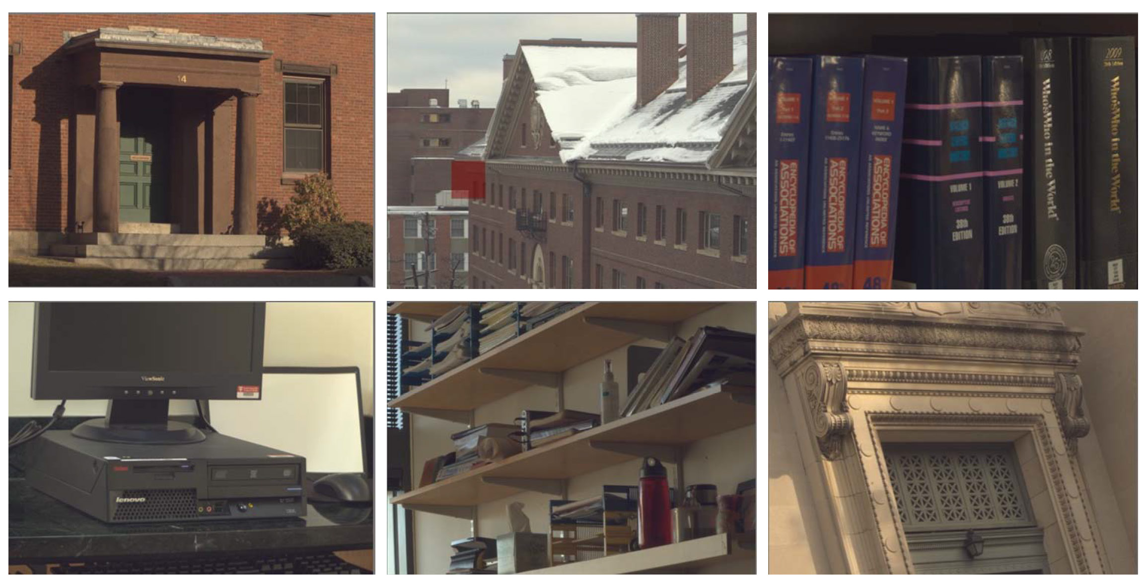
The spectral images in the Harvard Dataset are acquired using a CRI Nuance FX spectral camera with a liquid crystal tunable filter for spectral scanning. The spectral range is from 420nm to 720nm with 31 spectral bands. The Harvard Dataset consists of 50 spectral images with distinct natural scenes. In the experiments, 6 deteriorated spectral images with large-area saturated pixels are removed. 35 spectral images are randomly selected for training, and 9 spectral images are used for testing. The specific splitting can be checked in ./data/Harvard_Dataset.txt.

Click here to download Harvard Dataset.

1.Configurations

The configurations are the same as ICVL Dataset.

2.Results

Comparison of performance and complexity on Harvard Dataset (The ' indicates that the maximum pixel value used in the calculation of PSNR is 1.0)

Year	Method	Performance					Complexity
		Size	PSNR	SSIM	Source	Code Link	Params(M)	FLOPs(GMac)
2021	DRAN	256*256	35.690'	0.945	Original Paper	Private	/	/
2021	DEIL	512*512	34.052	0.984	Original Paper	Private	/	/
2021	DTLP	256*256	32.433	0.941	Original Paper	PyTorch TensorFlow	3.20	185.47
2020	DNU	512*512	32.710	0.978	Original Paper	PyTorch	4.21	1104.96
		512*512	32.550	0.977	Reproduced Paper
2019	DSSP	256*256	37.620'	0.955	Reproduced Paper	TensorFlow	0.334	22.42
		512*512	32.840	0.979	Original Paper			89.68
2019	HyperR- econNet	256*256	36.040'	0.938	Reproduced Paper	PyTorch Caffe	3.86	393.12
		512*512	30.341	0.964	Original Paper			1572.48
2019	λ-Net	256*256	29.373	0.909	Reproduced Paper	TensorFlow	58.26	44.82
		512*512	29.279	0.950	Reproduced Paper			179.28
2019	DTLR	256*256	31.136	0.932	Reproduced Paper	Private	/	≥1000
2018	ISTA-Net	256*256	29.870	0.913	Reproduced Paper	PyTorch TensorFlow	3.12	32.53
		512*512	31.130	0.967	Reproduced Paper			130.12
2017	Autoe- ncoder	256*256	29.205	0.912	Reproduced Paper	TensorFlow	/	/
		512*512	30.300	0.952	Reproduced Paper
2017	3DNSR	256*256	28.638	0.903	Reproduced Paper	Private	/	≥1000
		512*512	28.508	0.940	Reproduced Paper
2017	HSCNN	256*256	27.603	0.895	Reproduced Paper	Private	/	/
		256*256	35.090'	0.936	Reproduced Paper
		512*512	28.548	0.944	Reproduced Paper
2016	LRMA	256*256	30.499	0.930	Reproduced Paper	Private	/	≥1000
		512*512	29.680	0.952	Reproduced Paper
		512*512	30.113	0.957	Reproduced Paper
2016	AMP	512*512	26.670	0.935	Reproduced Paper	Private	/	≥1000
2011	ADMM	512*512	26.350	0.924	Reproduced Paper	Private	/	≥1000
2007	GPSR	512*512	24.960	0.907	Reproduced Paper	Private	/	≥1000
2007	TwIST	256*256	26.228	0.889	Reproduced Paper	Python	/	≥1000
		512*512	27.163	0.924	Reproduced Paper

CAVE&KAIST Datasets

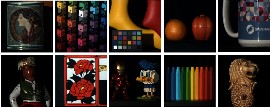
The spectral images in the CAVE Dataset are acquired using a VariSpec Liquid Crystal Tunable Filter and a Apogee Alta U260 CCD Camera. The spectral range is from 400nm to 700nm, which is divided into 31 spectral bands with approximate 10nm bandwidth for each band. There are 32 spectral images in CAVE Dataset.

The spectral images in the KAIST Dataset are acquired using a VariSpec Liquid Crystal Tunable Filter and a Pointgrey Grasshopper 9.1MP Monochromatic Camera. The spectral range is from 400nm to 720nm. There are 30 spectral images in KAIST Dataset.

In the experiments, 30 spectral images of CAVE Dataset are selected for training. 10 cropped spectral images with the size of 256 * 256 * 28, following the work of Meng et al., are selected for testing. The file list can be checked in ./data/CAVE&KAIST_Dataset.txt.

Click here to download CAVE Dataset. Click here to download KAIST Dataset.

1.Configurations

In this stage, the coded aperture pattern is a real mask with the size of 256 * 256, provided by Meng et al.. The file can be downloaded from this LINK. The other details of the simulation are the same as ICVL Dataset.

2.Results

Comparison of performance and complexity on KAIST Dataset

Year	Method	Performance				Complexity
		PSNR	SSIM	Source	Code Link	Params(M)	FLOPs(GMac)
2022	DAUHST	38.36	0.97	Original Paper	PyTorch	6.15	79.50
2022	BIRNAT	36.14	0.97	Original Paper	PyTorch	4.40	3536.64
2022	S^2-Transformer	36.48	0.96	Original Paper	Private	1.80	27.21
2022	CST	36.12	0.96	Original Paper	PyTorch	3.00	40.10
2022	GAP-CCoT	35.26	0.95	Original Paper	PyTorch	8.04	95.60
2022	MST	35.18	0.95	Original Paper	PyTorch	2.46	31.40
2022	HDNet	34.34	0.96	Original Paper	PyTorch	2.37	159.06
2022	CAE-SRN	33.26	0.93	Original Paper	PyTorch	1.25	83.06
2021	HerosNet	34.45	0.97	Original Paper	PyTorch	11.75	447.18
2021	DTLP	33.88	0.93	Original Paper	PyTorch TensorFlow	3.16	182.98
2021	DGSMP	32.63	0.92	Original Paper	PyTorch	3.76	647.80
2021	PnP-DIP-HSI	31.30	0.90	Original Paper	PyTorch	33.85	≥3000
2021	PnP-HSI	25.67	0.70	Reproduced Paper	PyTorch	1.96	≥3000
2020	GAP-Net	32.13	0.92	Original Paper	PyTorch	4.27	84.08
		32.47	0.93	Reproduced Paper
2020	TSA-Net	30.15	0.89	Original Paper	PyTorch	44.25	135.12
		31.46	0.89	Reproduced Paper
2020	DNU	30.74	0.86	Reproduced Paper	PyTorch	4.47	293.90
2019	DSSP	30.35	0.85	Reproduced Paper	TensorFlow	0.30	20.14
		28.93	0.83	Reproduced Paper
		32.39	0.97	Original Paper
2019	λ-Net	28.53	0.84	Reproduced Paper	TensorFlow	58.25	44.59
		29.25	0.89	Reproduced Paper
2019	DeSCI	25.27	0.72	Reproduced Paper	MATLAB	/	≥1000
		25.86	0.79	Reproduced Paper
2016	GAP-TV	24.36	0.70	Reproduced Paper	Python	/	≥1000
		23.73	0.68	Reproduced Paper
2007	TwIST	23.12	0.67	Reproduced Paper	Python	/	≥1000
		22.44	0.70	Reproduced Paper

Welcome

If you think there is any false, omissions or other materials should be supplemented, please contact us!