Install ebirdst from CRAN with:
install.packages("ebirdst")
Alternatively, you can install the development version from GitHub with:
# install.packages("remotes")
remotes::install_github("CornellLabofOrnithology/ebirdst")
The current version of ebirdst is designed for working with the eBird
Status and Trends data estimated for 2018. Older versions of the Status
and Trends data can be accessed by installing the associated version of
ebirdst from GitHub. For example, 2016 estimates, corresponding to
v0.1.0 of this package, can be accessed with:
# install.packages("remotes")
remotes::install_github("CornellLabofOrnithology/ebirdst@v0.1.0")
If you use the the eBird Status & Trends data please cite it with:
Fink, D., T. Auer, A. Johnston, M. Strimas-Mackey, O. Robinson, S. Ligocki, B. Petersen, C. Wood, I. Davies, B. Sullivan, M. Iliff, S. Kelling. 2020. eBird Status and Trends, Data Version: 2018; Released: 2020. Cornell Lab of Ornithology, Ithaca, New York. https://doi.org/10.2173/ebirdst.2018
For a full introduction and advanced usage, please see the package website. An introductory vignette details the data access and structure of the results. An intro mapping vignette expands upon the quick start readme and shows the basic mapping moves. The advanced mapping vignette shows how to reproduce the seasonal maps and statistics on the eBird Status and Trends website. Finally, the non-raster data vignette details how to access additional information from the model results about predictor importance and directionality, as well as predictive performance metrics.
To access old versions of the vignettes suitable for working with
previous eBird Status and Trends releases go to the versions page of
the GitHub
repository.
Download and unzip the source code for the release associated with the
version of the data you want to work with. Opening the file
docs/index.html will open the package website for this version, which
gives access to all the documentation and vignettes.
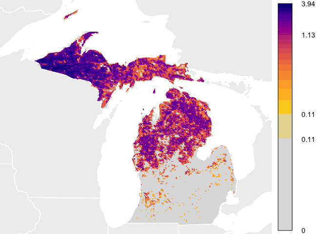
This quick start guide shows how to download data and plot abundance
values similar to how they are plotted for the eBird Status and Trends
Abundance
animations.
In this guide, a simplified example dataset is used consisting of
Yellow-bellied Sapsucker in Michigan. For a full list of the species
available for download, look at the data frame ebirst_runs, which is
included in this package.
Important note: after downloading the results, do not change the file structure. All functionality in this package relies on the structure inherent in the delivered results. Changing the folder and file structure will cause errors with this package. If you use this package to analyze the results, you do not ever need to interact with the files directly, outside of R.
library(ebirdst)
library(viridis)
library(raster)
library(sf)
library(rnaturalearth)

# download data
# download a simplified example dataset from aws s3
# example data are for yellow-bellied sapsucker in michigan
# by default files will be stored in a persistent data directory:
# rappdirs::user_data_dir("ebirdst"))
sp_path <- ebirdst_download(species = "example_data")

# load estimated relative abundance and label with dates
# this raster stack has 52 layers, one for each week of the year
abunds <- load_raster("abundance", path = sp_path)

# use parse_raster_dates() to get actual date objects for each layer
date_vector <- parse_raster_dates(abunds)
print(date_vector)
#>  [1] "2018-01-04" "2018-01-11" "2018-01-18" "2018-01-25" "2018-02-01" "2018-02-08" "2018-02-15"
#>  [8] "2018-02-22" "2018-03-01" "2018-03-08" "2018-03-15" "2018-03-22" "2018-03-29" "2018-04-05"
#> [15] "2018-04-12" "2018-04-19" "2018-04-26" "2018-05-03" "2018-05-10" "2018-05-17" "2018-05-24"
#> [22] "2018-05-31" "2018-06-07" "2018-06-14" "2018-06-21" "2018-06-28" "2018-07-06" "2018-07-13"
#> [29] "2018-07-20" "2018-07-27" "2018-08-03" "2018-08-10" "2018-08-17" "2018-08-24" "2018-08-31"
#> [36] "2018-09-07" "2018-09-14" "2018-09-21" "2018-09-28" "2018-10-05" "2018-10-12" "2018-10-19"
#> [43] "2018-10-26" "2018-11-02" "2018-11-09" "2018-11-16" "2018-11-23" "2018-11-30" "2018-12-07"
#> [50] "2018-12-14" "2018-12-21" "2018-12-28"

# select a week in the summer
abund <- abunds[[26]]
rm(abunds)

# project to mollweide for mapping
# the nearest neighbor method preserves cell values across projections
mollweide <- "+proj=moll +lon_0=-90 +x_0=0 +y_0=0 +ellps=WGS84"
abund_moll <- projectRaster(abund, crs = mollweide, method = "ngb")

# get reference data from the rnaturalearth package
# the example data currently shows only the US state of Michigan
wh_states <- ne_states(country = c("United States of America", "Canada"),
                    returnclass = "sf") %>%
  st_transform(crs = mollweide) %>%
  st_geometry()

# calculate ideal color bins for abundance values for this week
week_bins <- calc_bins(abund_moll)

# start plotting
par(mfrow = c(1, 1), mar = c(0, 0, 0, 6))

# use raster bounding box to set the spatial extent for the plot
bb <- st_as_sfc(st_bbox(trim(abund_moll)))
plot(bb, col = "white", border = "white")

# add background reference data
plot(wh_states, col = "#eeeeee", border = NA, add = TRUE)

# plot zeroes as gray
plot(abund_moll == 0, col = "#dddddd",
     maxpixels = ncell(abund_moll),
     axes = FALSE, legend = FALSE, add = TRUE)

# define color bins
qcol <- abundance_palette(length(week_bins$bins) - 1, "weekly")

# plot abundances
plot(abund_moll, col = qcol, breaks = week_bins$bins,
     maxpixels = ncell(abund_moll),
     axes = FALSE, legend = FALSE, add = TRUE)

# for legend, create a smaller set of bin labels
bin_labels <- format(round(week_bins$bins, 2), nsmall = 2)
bin_labels[!(bin_labels %in% c(bin_labels[1],
                               bin_labels[round((length(bin_labels) / 2)) + 1],
                               bin_labels[length(bin_labels)]))] <- ""
bin_labels <- c("0", bin_labels)

# create colors that include gray for 0
lcol <- c("#dddddd", qcol)

# set legend such that color ramp appears linearly
ltq <- seq(from = week_bins$bins[1], to = week_bins$bins[length(week_bins$bins)],
           length.out = length(week_bins$bins))
ltq <- c(0, ltq)

# plot legend
plot(abund_moll ^ week_bins$power, legend.only = TRUE,
     col = lcol,
     breaks = ltq ^ week_bins$power,
     lab.breaks = bin_labels, legend.shrink = 0.97,
     legend.width = 2, axis.args = list(cex.axis = 0.9, lwd.ticks = 0))

# add state boundaries on top
plot(st_geometry(wh_states), add = TRUE, col = NA, border = "white", lwd = 1.5)

