ESTIpop

ESTIpop is an R-wrapped C++ package to simulate and estimate the parameters of continuous-time Markov branching processes with time-dependent rates.

Installation Notes

Dependencies

GNU Scientific Library
- (OSX) brew install gsl with Homebrew or from (http://ftpmirror.gnu.org/gsl/).
- (Windows) download and extract the file local###.zip and create an environmental variable LIB_GSL to add the directory (see notes about Windows installation below for more details).
- (Linux) install libgsl0-dev and gsl-bin.
Rtools (Windows only)
devtools

Important notes about Windows installation

Rtools contains the necessary resources to compile C++ files when installing packages in R. GSL is also required which can be downloaded from (http://www.stats.ox.ac.uk/pub/Rtools/goodies/multilib/local323.zip). After downloading, unzip to your R directory. Depending on if your computer is 32 or 64-bit, move the library files from local###/lib/i386 (32-bit) or local###/lib/x64 (64-bit) to local###/lib.

To set the environmental variable LIB_GSL on a Windows 7/10 computer, go to “Advanced system settings” in Control Panel > System and Security > System and click Environmental Variables. Create a new system variable with

Variable Name: LIB_GSL
Variable Value: “C:/path/to/local323” (include quotes)

Recommended R packages

ggplot2
R.utils

Installation

To install in R, type:

install.packages("devtools")
devtools::install_git("https://github.com/Michorlab/estipop.git")

Uses

Estimation

ESTIpop is an R package that estimates the parameters of continuous-time Markov branching processes (CTMBPs) with constant or time-dependent rates. A CTMBP is a stochastic process in which individuals live for a random amount of time before generating some number of offspring, each of which continues the process. Individuals can belong to one of a finite number of types. Each type has its own continuous lifetime distribution, as well a distirbution that governs the number and types of offspring it produces. The process is Markov because an individual’s remaining lifetime is independent of the individual’s age. However, the rates at which individuals die and reproduce can still vary with time, analogous to the nature of arrivals in a time-inhomogenous Poisson process.

Simulation

ESTIpop also provides methods to simulate continuous-time Markov branching processes. Simulated processes can have arbitrary numbers of types and transitions, and may have rates which are constant or time-dependent.

Objects in ESTIPop

ESTIpop uses a common representation of branching process models for simluation and estimation. A branching process model is represented by a process_model object containing one or more transition objects, and each transition object is associated with a rate object.

rate Objects

A rate object represents the rate at which some event occurs, and may be a function of time and multiple other parameters. The constructor rate(exp) takes an R expression which describes how the rate depends on time and other parameters. For example:

r1 = rate(3.5) # a constant, known rate
r2 = rate(2*t) # a rate which increases linearly with time
r3 = rate(1.5*params[1]) #a rate which depends on one unknown parameter
r4 = rate(params[1] + params[2]*exp(-.5*t)) # a rate which depends on 2 unknown 
                                            # parameters and time

It is important to note that the variable t and the params vector are not variables which we have defined previously in the program. The rate constructor acts on an expression which encodes how the rate evolves with time and various other parameters. We will be able to evaluate this expression later when we plug in parameter values at a specific time.

The rate constructor expects expressions which conform to the following subset of the R grammar, and will throw an error at other inputs.

Type	Allowed Symbols
Unary Operators	+ - ()
Binary Operators	+ - / * > >= < <=
Functions	sin(), cos(), log(), exp()
names	params[i], t
numerics	any scalar numeric value

transition Objects

A transition object represents a type of birth or death event which can occur in the branching process model. A transition object has 3 attibutes:

parent: The type of the parent which dies and is removed from the population when the transition occurs
offspring: The number of each type of offspring which are produced in the transition. This should be an d-length vector where d is the number of types in the population.
rate: A rate object (described above) governing how quickly this transition occurs

A transition object can be constructed as follows:

r = rate(.5*params[1] + params[2]*exp(-t))
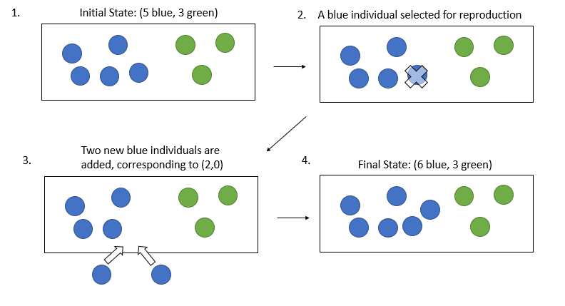
#a type 2 parent dies and produces 2 offspring of different types
trans = transition(rate = r, parent = 1, offspring = (2,0))

This transition is illustrated in the following figure:

process_model Objects

A process_model object is a collection of transition objects which together make up a branching process system. A process_model object is constructed from a sequence of transition objects which can occur in the system. All of the transition objects must assume the same number of types, and the process_model constructor will throw an error if this is not the case.

#simple one-type birth death model with rates that decay exponentially over time
birth = rate(params[1]*exp(-params[3]*t))
death = rate(params[2]*exp(-params[3]*t))
model = process_model(transition(rate = birth, parent = 1, offspring = 2),
                      transition(rate = death, parent = 1, offspring = 0))

Note that model still retains all of the time- and parameter-dependence of its constituent transitions. Also notice that, since params[3] was used in both the birth and death rate, this model has the constraint that birth and death rates decay at equal speed.

Simulation

Armed with a process_model object, ESTIpop allows for the simulation of this system under various parameters values. ESTIpop uses C++ for high-performance simulation. In the case of time-dependent rates, ESTIpop parses the expressions and translates them into dynamically loaded C++ code.

The branch function is used to simulate the system specified by a process_model object. It’s parameters are as follows:

Argument	Type	Description	Optional?
`model`	`process_model` object	The system to simulate	No
`params`	numeric vector	The parameters to plug into the system during simulation	No
`init_pop`	numeric vector	The population at the start of the simulation (time 0)	No
`time_obs`	numeric vector	The timepoints at which to record the state of the population	No
`reps`	numeric scalar	The number of times to run the simulation	No
`silent`	logical	Whether to silence intermediate printouts form the C++ simulator	Yes
`keep`	logical	Whether to keep logs files from the C++ simulation	Yes
`seed`	logical	A seed for the random number generator	Yes

The following examples demonstrate ESTIPop’s simulation features:

One-Type Birth-Death Process

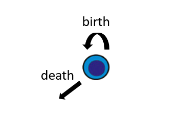
We’ll start by simulation the one-type birth-death model shown in the following figure. In this model, a population of a single type experiences birth events, in which an individual from the population is chosen to replicate, and death events, in which an individual from the population is chosen for removal. To test our estimation procedure, we begin by simulating data using functions available in ESTIpop. We initiate the population with size 100 and allow it expand for 5 units of time with birth parameter 1 and death parameter 0.7. Using the following code, we generate 1,000 samples from this process.

library(estipop)

#Create a one-type birth-death model where the birth rate increases over time
model = process_model(transition(rate = rate(params[1] - params[2]*exp(-params[3]*t)), 
                                 parent = 1, offspring = 2),
                      transition(rate = rate(params[4]), parent = 1, offspring = 0))

#Specify the time points at which we will record the state of the simulation
time = seq(0,20,.5)

#The initial size of the simulated population
init_pop = c(500)

#Parameters to plug into the model for this simulation run
params = c(.3,.25,.1, .2)  

#Numer of times to run the simulation
reps <- 1000

res = branch(model = model, params = params, init_pop = init_pop, 
             time_obs = time, reps = reps)

#Plot a single replication of the simulation
single <- dplyr::filter(res, rep == 1)
plot(single$time, single$type1, xlab = "time", ylab = "population size")

res now contains a dataframe with the result of the simulation. We can now analyze the results of the simulation.

res <- dplyr::filter(res, time == 20) #just take the last timepoint
#compute the theoretical moments of the population distribution
mom <- compute_mu_sigma(model, params, 0, 20, init_pop)

print(paste("Sample Mean: ", mean(res$type1)))

## [1] "Sample Mean:  426.535"

print(paste("True Mean: ", mom$mu))

## [1] "True Mean:  425.364259883693"

print(paste("Sample Variance: ", var(res$type1)))

## [1] "Sample Variance:  4502.39116616617"

print(paste("True Variance: ", mom$Sigma))

## [1] "True Variance:  4386.38004944714"

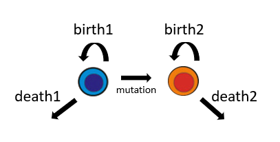
Two-Type Birth-Death-Mutation Process

We now consider the two-type process shown in the following figure. Here, each of the two population types has separate birth and death rates, as well a mutation rate from the type 1 population to the type 2 population. We’ll again simulate 1000 examples and compare the results with the theoretical moments.

library(estipop)

time = 5
init_pop= c(100, 0)

params = c(.4,.1,.7,.1, .3)

#time-homogenous two-type model
model = process_model(transition(rate = rate(params[1]), parent = 1, offspring = c(2,0)),
                      transition(rate = rate(params[2]), parent = 1, offspring = c(0,0)),
                      transition(rate = rate(params[3]), parent = 2, offspring = c(0,2)),
                      transition(rate = rate(params[4]), parent = 2, offspring = c(0,0)),
                      transition(rate = rate(params[5]), parent = 1, offspring = c(1,1)))

res = branch(model, params, init_pop, time, 1000)

Now we analyze the simulation results and compare them with theory

mom = compute_mu_sigma(model, params, 0, 5, init_pop)
print(paste("Sample Mean: ", toString(c(mean(res$type1), mean(res$type2)))))

## [1] "Sample Mean:  448.151, 1571.425"

print(paste("True Mean: ", toString(mom$mu)))

## [1] "True Mean:  448.168943658686, 1560.38542784701"

print(paste("Sample Variance: ", toString(c(var(res$type1), var(res$type2)))))

## [1] "Sample Variance:  2756.96316216216, 41241.8542292292"

print(paste("Sample Covariance:", cov(res$type1, res$type2)))

## [1] "Sample Covariance: 4801.0769019019"

print(paste("True Variance: ", toString(diag(mom$Sigma))))

## [1] "True Variance:  2600.64200784677, 39457.2214316809"

print(paste("True Covariance: ", toString(mom$Sigma[1,2])))

## [1] "True Covariance:  4527.31533883025"

Estimation

Given process_model object and a set of datapoints generated from that model, ESTIpop can estimate the model’s unknown parameter values.

The estimate and estimate_td functions are used to estimate the parameters of process_model object. The arguments these function as as follows:

Argument	Type	Description
`model`	`process_model` object	The system whose parameters are being estimated
`init_pop`	`N` x `d` matrix	The initial population in each of the observations in the dataset
`final_pop`	`N` x `d` matrix	The final observed population in each observation
`start_times`	`N` x 1 vector	The time at which each entry in `init_pop` was observed
`end_times`	`N` x 1 vector	The time at which each entry in `final_pop` was observed
`initial_ params`	`m` x 1 vector	The parameter values at which to initialize the estimation procedure
`lower`	`m` x 1 vector	Lower bounds on each parameter to be estimated
`upper`	`m` x 1 vector	Uppose bounds on each parameter to be estimated
`trace`	logical	Whether to enable output during optimization

The estimate function is a wrapper for the estimate_td function. estimate only requires the elapsed time between the initial and final obervations of each entry in the dataset, rather then the exact times of each observation. estimate can be used when the rates of a model do not depend on time.

The following examples demonstrate ESTIPop’s estimation features:

Time-dependent one-type model

We now return to the one-type time-dependent model explored in the simulation section. In this model the birth rate declines as an unknown exponential function while the death rate remains constant. This could represent the dynamics of a population recovering from a drug for which we want to estimate a pharmacokinetic model. First we will simulate the model, this time with far fewer replications:

library(estipop)

#Create a one-type birth-death model where the birth rate increases over time
model = process_model(transition(rate = rate(params[1] - params[2]*exp(-params[3]*t)), 
                                 parent = 1, offspring = 2),
                      transition(rate = rate(params[4]), parent = 1, offspring = 0))

#Specify the time points at which we will record the state of the simulation
time = seq(0,20,1)

#The initial size of the simulated population
init_pop = c(500)

#Parameters to plug into the model for this simulation run
params = c(.3,.25,.1, .2)  

#Numer of times to run the simulation
reps <- 20

res = branch(model = model, params = params, init_pop = init_pop, 
             time_obs = time, reps = reps)
simdat <- format_sim_data(res, ntypes = 1)

The last line converts the dataset into the format expected by our estimation functions. Note that, because the process is Markov, we can compute the likelihood of the entire dataset by computing the likelihood of each observation conditioned on the previous observation. We now estimate the parameters of the model:

est = estimate_td(model, init_pop = simdat$type1_prev, 
                  final_pop =simdat$type1,
                  start_times = simdat$prev_time, 
                  end_times = simdat$time,
                  initial = runif(4,0,.5), 
                  lower = rep(0,4),
                  upper = rep(.5,4),
                  method = "L-BFGS-B")

print(est$par)

## [1] 0.2632411 0.2414000 0.1098404 0.1774179

After estimation we recover parameter values very close to ground truth.

Time-homogenous birth-death-mutation model

We’ll now estimate the parameters of the two-type birth-death-mutation model we simulated earlier.

time = seq(0,10,1) 
initial = c(100, 0)

params = c(.4,.1,.7,.1, .3)

model = process_model(transition(rate = rate(params[1]), parent = 1, offspring = c(2,0)),
                      transition(rate = rate(params[2]), parent = 1, offspring = c(0,0)),
                      transition(rate = rate(params[3]), parent = 2, offspring = c(0,2)),
                      transition(rate = rate(params[4]), parent = 2, offspring = c(0,0)),
                      transition(rate = rate(params[5]), parent = 1, offspring = c(1,1)))



res = branch(model, params, initial, time, 30)
simdata = format_sim_data(res, model$ntypes)
est = estimate(model, init_pop = cbind(simdata$type1_prev, simdata$type2_prev), 
               final_pop = cbind(simdata$type1, simdata$type2),
               times = simdata$dtime,
               initial = runif(5,0,.5),
               lower = rep(1e-5,5),
               upper = rep(1,5),
               method = "L-BFGS-B")

print(est$par)

## [1] 0.4084356 0.1097101 0.6591385 0.0601875 0.3050673

Once again we estimate values close to ground truth.

Two-Type Drug Resistance Model (Four Types)

The two-type drug resistance model is a four-type process in which two types of mutation are possible. The type 0 population harbors no mutations, the type 1 population harbors mutation 1, the type 2 population harbors mutation 2, and the type 12 population harbors both mutations 1 and 2. Each type undergoes birth and death events, as well as the possibility for further mutation as illustrated in the following figure.

We now simulate and estimate this model. To reduce the number of parameters, we assume that all types share the same death rate.

time = seq(0,10,1) 
initial = c(100, 0,0,0)

params = c(.4,.7,.5,.2,.3,.1,.4,.3, .3)

model = process_model(
  transition(rate = rate(params[1]), parent = 1, offspring = c(2,0,0,0)),
  transition(rate = rate(params[2]), parent = 2, offspring = c(0,2,0,0)),
  transition(rate = rate(params[3]), parent = 3, offspring = c(0,0,2,0)),
  transition(rate = rate(params[4]), parent = 4, offspring = c(0,0,0,2)),
  transition(rate = rate(params[5]), parent = 1, offspring = c(1,1,0,0)),
  transition(rate = rate(params[6]), parent = 1, offspring = c(1,0,1,0)),
  transition(rate = rate(params[7]), parent = 2, offspring = c(0,1,0,1)),
  transition(rate = rate(params[8]), parent = 3, offspring = c(0,0,1,1)),
  transition(rate = rate(params[9]), parent = 1, offspring = c(0,0,0,0)),
  transition(rate = rate(params[9]), parent = 2, offspring = c(0,0,0,0)),
  transition(rate = rate(params[9]), parent = 3, offspring = c(0,0,0,0)),
  transition(rate = rate(params[9]), parent = 4, offspring = c(0,0,0,0)))


res = branch(model, params, initial, time, 30)
simdata = format_sim_data(res, model$ntypes)
init_pop = cbind(simdata$type1_prev, simdata$type2_prev,
                 simdata$type3_prev, simdata$type4_prev)
final_pop = cbind(simdata$type1, simdata$type2,
                  simdata$type3, simdata$type4)

est = estimate(model, init_pop = init_pop,
               final_pop = final_pop, 
               times = simdata$dtime,
               initial = rbeta(9,2,1),
               lower = rep(1e-5,9),
               upper = rep(1,9),
               method = "L-BFGS-B")

print(est$par)

## [1] 0.3882471 0.6848637 0.4824548 0.1992096 0.2986555 0.1032464 0.3927194 0.3187989 0.2878569

Once again, our estimates agree closely with ground truth.