Investigating the Robustness of RDF2Vec

In times of semantic web there is much data available in the form of knowledge graphs. However, as many machine learning algorithms rely on numeric data, it is required to transform the data from the space of graphs to a (for instance) euclidean space to execute downstream tasks. We call a numeric representation of the entities in a graph a graph embedding.

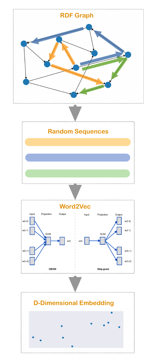
There are various different techniques to embed a graph, see for instance [1] for a brief overview. One popular embedding technique is called RDF2Vec [2], which transforms a RDF graph based on random traversions on the graph. One specific form of RDF2Vec collects random walks on the graph. These randomly generated sequences are interpreted as sentences, which can be used to create embeddings in the fashion of word2vec [3] [4]. The following figure visualizes the RDF2Vec algorithm:

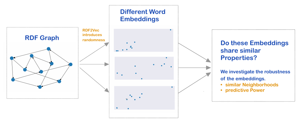
Consequentially, as the utilized sequences rely on random walks, RDF2Vec relies on randomness as well. With this in mind, my aim of the seminar work is to investigate whether this randomness harms the robustness of RDF2Vec. To do so, we randomly generate and compare K different embeddings of the same graph.

1. Notation

Let $E_1,...,E_K$ be $K$ different embeddings of a RDF graph into $\mathbb{R}^D$ (the D-dimensional real vector space) for some embedding dimension $D$. That is, each embedding is a matrix $E_k$ in $\mathbb{R}^{(N \times D)}$, where $N$ is the number of entities. Each row of $E_k$ represents the $D$-dimensional embedding of an entity.

2. How to investigate the Robustness of an Embedding?

After generating $K$ different embeddings, I need to find a metric that compares the similarity of the embeddings, which will serve as a measure of robustness of RDF2Vec. In this work, I introduce 2 ways to investigate the robustness.

2.1. The Neighborhood-Similarity

One way to measure the similarity of different embeddings is to compare the resulting neighborhoods of each entity. This is especially relevant for downstream clustering of the graphs entities.

To illustrate this concept, consider a 2-D word embedding, i.e. the entities of the graphs are mapped onto the 2-dimensional space $\mathbb{R}^2$. Assume that RDF2Vec generates 2 embeddings $E_1$ and $E_2$, where $E_2$ is a $90$ degrees rotated version of the first embedding $E_1$.

How similar are the embeddings? In terms of euclidean distance, the two embeddings might heavily differ from each other even though the different entities are, in relation to each other, at the same position. Our intuition would probably led us to the conclustion that clustering should yield the same result for both embeddings. In fact, many machine learning are also invariant under rotation and translation, such as the popular family of k-NN algorithms. These algorithms take the (euclidean) neighborhood of each data sample into account.

This leads us to the first measure of robustness, which aims to answer the question:

How similar are the neighborhoods for each embedded node that result from different iterations of RDF2Vec? That is, we want to investigate whether RDF2Vec preserves the neighborhoods across different iterations.

The first measure of robustness is then constructed as follows:

For 2 neighborhoods of the same node, we calculate the similarity between these as the Jaccard distance of the neighborhoods, that is, we take the intersection of both sets into relation to the union of both sets. This gives us a similarity score, which ranges from 0 to 1, of 2 neighborhoods.
We can then compute a similarity score of 2 embeddings by averaging the similarity of the 2 neighborhoods (step 1) over each node.
To obtain a similarity score of $K>2$ embeddings, we repeat step 2. for each pair of embeddings. Finally, the Neighborhood-Similarity of the embeddings $E_1,...,E_K$ is computed as the average over all pairwise similarities of $E_i$ and $E_j$.

2.2. The Predictive-Similarity

The second approach is based on the idea that similar embeddings should lead to similar predictions. In this case, we have several graph entities that belong to a specific class. For instance, the AIFB dataset (details in Section 4.2.) includes entities that describe a specific professor, which belongs to the class of academic stuff. One prediction task could be, given the graph embedding of an entity, to predict the entity class.

To be precise, given some embeddings $E_1, ..., E_K$ we want to train K classifier. Each of them is trained with the data (of a training subset of ) $E_1, ..., E_K$, respectively. Then, to compute the Predictive-Similarity of the embeddings, we investigate the similarity of the prediction results (on a test set of $E_1, ..., E_K$). The similarity of the predictions is simply measured as the average amount of equal predictions of the entities.

For illustration, consider the following simple example. We have 2 embeddings with $100$ entities. We train two classifier on the first $98$ representations of each embedding. To test the Predictive-Similarity, we investigate the resulting predictions of the last 2 representations. Assume that the first classifier outputs the class types "Academic Stuff" and "Publication" for the representations of entity 99 and 100. The second classifier outputs the class types "Academic Stuff" and "Academic Stuff" for the same entities. Hence, as only 1 of 2 predicitons is similar, we would assign these two embeddings a similarity score of $1/2$.
As in Section 2.1. we can then average the pairwise similarities over all embeddings to obtain a similarity score of $K>2$ embeddings. I chose a k-NN classfier with $k=20$.

3. The Embedding Dimension

The embedding dimension plays a crucial role for the representative power of an embedding. On the one hand, it is clear the an increment of the embedding dimension also increases the representational power of an embedding. However, there is a drawbacks connected to a big embedding dimension: Making the embedding space $\mathbb{R}^D$ small forces the algorithm to select more meaningful/structured representations. Hence, we usually do not want $D$ to be too large. However, letting $D$ be too small might be too restrictive as it gets 'harder' to fit all entities (in a meaningful manner) into the small space.

But more importantly, we must pay attention on the fact that weird stuff is happening in higher dimensions. For instance, [5] shows that euclidean distances ,which are used for the neighborhood-similarity, become, roughly said, 'meaningless' in higher dimensions. This is because the distance between entities in higher-dimension spaces converge to the same value. This phenomenon is quite unintuitive and leads to poor results in our evaluation.

Hence, I decided to employ the following pipeline:

Generate embeddings with $D=100$.
Employ a dimension reduction algorithm (PCA or t-SNE [6]), which maps the embedding to a 2- or 3-dimensional space.
Calculate the metrics from Section 2.1 and 2.2. on the 2- or 3-dimensional reduced embeddings.

4. Implementation

4.1. Software

Besides some standard libraries (numpy, pandas, sklearn, etc.) we employed

rdflib [7] to parse the RDF graphs;
pyrdf2vec [8] for a python implementation of RDF2Vec.

4.2. Data

Due to computational limitations, I investigated the following small sized data sets:

AIFB: Describes an research institute (AIFB) including its staff, research groups, publications, and so on [9].
MUTAG: Biological dataset that cotains information about molecules that are potentially carcinogenic [10].
BGS: (British Geological Survey) Contains geological measurements in Great Britain [11].

In the empirical analysis I employed the same hyper parameters as [2].

4.3. Installing

To install the required software simply run :

pip3 install -r requirements.txt

4.4. How the git is organized

The different programs are designed to be run in the following order: 0. cd code to switch to the code directory.

python generateEmbeddings.py to generate the embeddings. The user can choose between various parameters, see python generateEmbeddings.py -h.
python dim_reduction.py to apply a dimension reduction on the embeddings, see Section 3. The user can choose between various parameters, see python dim_reduction.py -h. To run the script for all possible configurations run python run_dimred.py.
python stability_analysis.py to run the stability analysis according to Section 2.1 (The Neighborhood-Similarity). The user can choose between various parameters, see python stability_analysis.py -h. To run the script for all possible configurations run python run_stab_ana.py.
The results that correspond to the Predicitve-Similarity from Section 2.2. can be accessed via the notebook (for instance using jupyter lab): jupyter lab prediction_class.ipynb.
python results.py to summarize the results in a table. In addition you can generate corresponding boxplots that depict the empirical distribution of similarities: python boxplots.py.

5. Result

For the stability analysis, we employed $K=10$ different embeddings. The following table shows the Neighborhood-Similarity of these embeddings. Note, that we used 2 variants of RDF2Vec, one that employs word2vec via skip-gram (sg), and the second one employs word2vec via cbow. For details, I refer to [2].

Neighborhood-sim.	AIFB (sg)	BGS (sg)	MUTAG (sg)	AIFB (cbow)	BGS (cbow)	MUTAG (cbow)
PCA2d	0.14	0.06	0.04	0.09	0.06	0.03
PCA3d	0.23	0.10	0.06	0.14	0.07	0.05
tSNE2d	0.40	0.26	0.19	0.35	0.16	0.11
tSNE3d	0.41	0.27	0.19	0.36	0.17	0.11

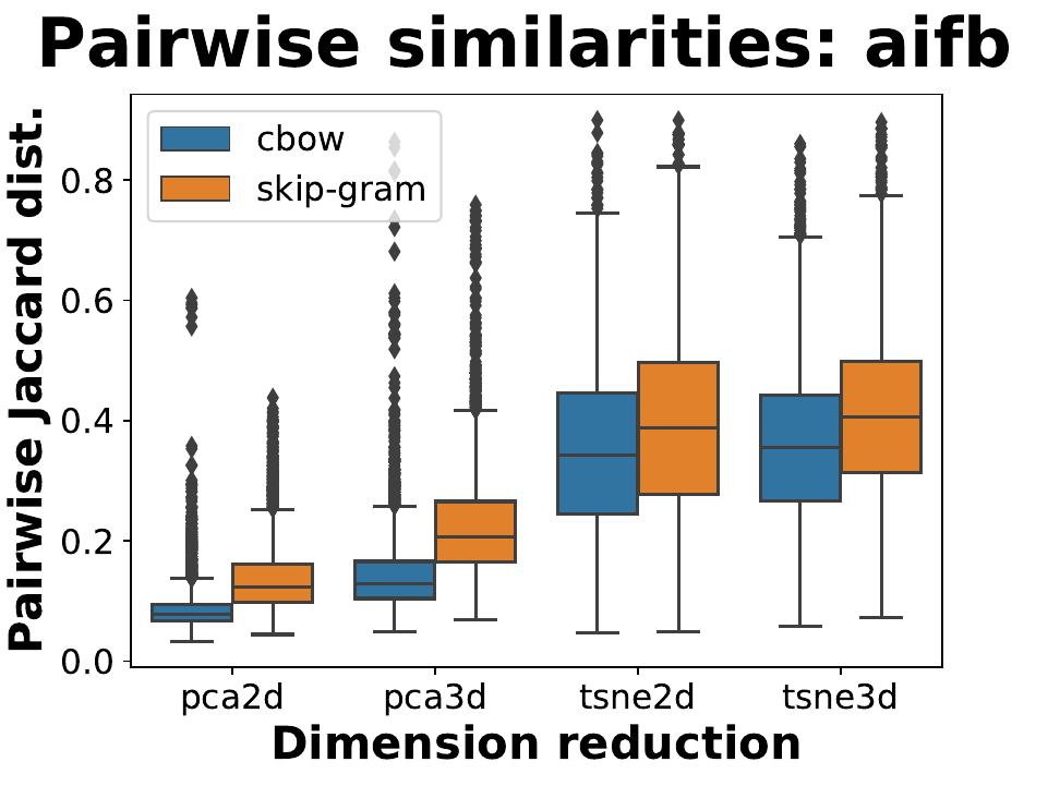
We observe that RDF2Vec is most stable when applied onto AIFB using t-SNE. Nonetheless, the robustness is still a bit disappointing since, in average, the neighborhoods are only 41% similar to each other. For the other 2 data sets, the robustness is much worse.

The following boxplot depicts the empirical distribution of similarities between neighborhoods.

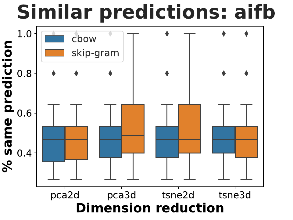
Finally, we plot a boxplot that depicts the Predictive-Similarity of each entity across the embeddings:

Importantly, note that I trimmed down the data such that we end up with a classification problem with only 3 classes. This is due to underrepresentation of various classes. In the case of AIFB, the class labels were "Publication", "Person", and "InProceedings". Again, we observe that the median performance swings around $0.5$, which is quite disappointing since we considered only a 3-label-classification problem.

6. Conclusion

RDF2Vec is a popular graph embedding technique, however due to the inclusion of random walks, it relies on randomness. To investigate the robustness of RDF2Vec in spite of the randomness, I introduced 2 measures for the similarity of various embeddings, the Neighborhood-Similarity and the Predictive-Similarity. The final results in Section 5. seemingly lead to the conclusion that RDF2Vec fails to produce robust embeddings. This is true in my investigated setting. However, I must emphasize that there are some important things to point out:

I analyzed the robustness of the reduced embeddings (via dimension reduction). Hence, the dimension reduction algorithms might be a reason for the bad performance in terms of robustness. Especially as t-SNE itself relies on randomness.
On the other hand, analyzing the similarity in the 100-dimensional embedding space also did not lead to good results. But this is probably because euclidean neighborhoods are not a suitable measure for similarity in high-dimensional spaces.

Therefore, interesting follow-up works might be a) to investigate the robustness when RDF2Vec directly embeds the graph into a low-dimensional space, or b) to investigate the robustness in the high-dimensional space, $\mathbb{R}^100$ for instance, but using a better-suited similarity measure for these spaces, see [12].

References

[1] Wang, Q., et al. (2017). Knowledge graph embeddings: A survey of approaches and applications. IEEE Transactions on Knowledge and Data Engineering.

[2] Ristoski, P., Paulheim, H. (2016). Rdf2vec: Rdf graph embeddings for data mining. International Semantic Web Conference.

[3] Mikolov, T., et al. (2013). Distributed representations of words and phrases and their compositionality. Neural information processing systems.

[4] Mikolov, T., et al. (2013). Efficient estimation of word representations in vector space. arXiv preprint arXiv:1301.3781.

[5] Giraud, C. (2014). Introduction to high-dimensional statistics, Section 1. CRC Press.

[6] van der Maaten, L. (2008). Visualizing Data using t-SNE. Journal of Machine Learning Research.

[7] https://github.com/RDFLib/rdflib

[8] Vandewiele, G., et al. (2020). pyRDF2Vec: Python Implementation and Extension of RDF2Vec.

[9] Bloehdorn, S., Sure, Y. (2007). Kernel methods for mining instance data in ontologies. Proceedings of the 6th International The Semantic Web and 2Nd Asian Conference on Asian Semantic Web Conference.

[10] http://dl-learner.org

[11] http://data.bgs.ac.uk/

[12] Hinneburg, A., et al. (2000). What is the nearest neighbor in high dimensional spaces? International Conference on Very Large Data Bases.

MikeLasz/robustness_rdf2vec