PerishableDCM

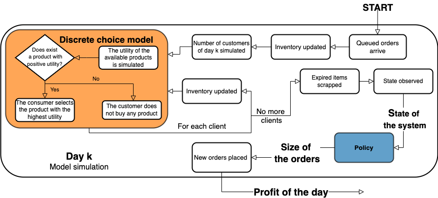
This library simulates the inventory control problem of perishable products by means of Discrete Choice Methods (DCM).

Specifically, PerishableDCM is a simulation environment for the management of perishable items with lead times and a fixed shelf life. It deals with multiple items, where orders for fresh products are issued each day. The product characteristics are:

The price at which items are purchased (C)
The price at which items are sold (P)
The salvage value (if any), when the items are scrapped (MD)

Demand is uncertain and subject to daily seasonality. The objective is to maximize the long-run average daily profit, but the software provides insights into the generated waste as well.

Structure of the code

|____envs
| |______init__.py
| |____dailySimulation.py
|____configurations
| |____conf_Products.json
| |____conf_Store.json
|____managers
| |______init__.py
| |____CustomerManager.py
| |____SupplyManager.py
| |____ScenarioGeneratorRandom.py
| |____StatManager.py
| |____InventoryManager.py
|____main_example.py

Dynamics of the simulation

The dynamics of the simulation of one day is hereafter represented.

Available features

Two dictionaries drive the parameters of the simulation: conf_Products and conf_Store, setting the features of the available products and of the store that sells them.

For example:

{
"A":{
    "LT":3,
    "SL":4,
    "P":[6,6,6,6],
    "C":3,
    "MD":0,
    "Q":[22.5,23,23.5,24]
},
"B":{
    "LT":2,
    "SL":2,
    "P":[3.3,4],
    "C":2,
    "MD":0,
    "Q":[18,20]
}
}

defines two products A and B, where B has:

A lead time of 2 days.
A shelf life of 2 days.
A price that decreases w.r.t. to the age (4 if new, 3.3 after one day).
A cost of 2.
No salvage value.
A quality (Needed for the linear DCM) that decreases w.r.t. the age (20 if new, 18 after one day).

Whereas, the conf_Store

{
"Seasonals":[90,100,100,100,130,200,200],
"ev_Daily":300,
"std_Daily":20,
"Distr":"Poisson",
"DCM":{
    "Type":"LinearBeta",
    "alpha":2,
    "beta":3
}
}

defines:

The seasonality that will be normalized by the software s.t. it will sum to 7.
The expected value of the number of clients per day.
The std of the number of clients per day.
The distribution employed to sample the number of clients (Currently Poisson and Normal are available).
The DCM and its peculiar requirements (currently only the linear DCM is available).

Example

A main_example file implements a constant policy through the gym OpenAI syntax.

The debug flag

flagPrint = True

provides insight into each step of the simulation. E.g.,

 day 407 
 inventory:
Product A : Stored
         0.0 items with  1 Residual shelf life
         0.0 items with  2 Residual shelf life
         101.0 items with  3 Residual shelf life
Product B : Stored
         19.0 items with  1 Residual shelf life
 onOrder:
Product A :Waiting for
         160.0  items A have just arrived.
         160.0  items, expected in 1 days
         160.0  items, expected in 2 days
         160.0  items, expected in 3 days
Product B :Waiting for
         100.0  items B have just arrived.
         100.0  items, expected in 1 days
         100.0  items, expected in 2 days
Total demand (partially lost):  235.0
Product  A  Ordered:  160  Sold:   [ 0.  0.  0. 71.]  Scrapped:  0.0
Product  B  Ordered:  100  Sold:   [19. 96.]  Scrapped:  0.0
 No purchase:  49 Unmet Demand:  0
Total unmet so far 6655
Total ordered so far  105820.0
Total scrapped so far 13459.0
Total sold so far [50991. 40496.]
Average profit 454.7299999999998
Profit of the day  192.7
State observation:  {'A': array([160., 160., 160.,  89., 101.,   0.]), 'B': array([100., 100.,   4.]), 'Day': 2}
Press Enter to continue

The state observation for each product is here made of the number of expected items subject to the lead time, concatenated with the number of stored items, divided by their residual shelf life.

Requirements

Name		Version employed	Description	Website
gym	>=	0.23.1	Toolkit for developing and comparing reinforcement learning algorithms	https://github.com/openai/gym

Citing Us

For more detailed information, this code is supported by two different articles that we recommend to cite in case you use the library.

@article{gioia2023simulation,
	title={Simulation-based inventory management of perishable products via linear discrete choice models},
  	author={Gioia, Daniele Giovanni and Felizardo, Leonardo Kanashiro and Brandimarte, Paolo},
  	journal={Computers \& Operations Research},
  	pages={106270},
  	volume = {157},
  	year={2023},
  	publisher={Elsevier}
}

@article{Gioia22Nantes,
	author = {Gioia, Daniele Giovanni and Felizardo, Leonardo Kanashiro and Brandimarte, Paolo},
	journal = {IFAC-PapersOnLine},
	number = {10},
	pages = {2683-2688},
	note = {10th IFAC on Manufacturing Modelling, Management and Control MIM 2022},
	title = {Inventory management of vertically differentiated perishable products with stock-out based substitution},
	volume = {55},
	year = {2022} }

${\color{red}{\text{Typos}}}$ on 'Simulation-based inventory management of perishable products via linear discrete choice models'

Please notice that in Eq.(10) and Eq.(12) of the article, sums range over the following values:

$$\sum_{l=0}^{\mathsf{LT}_j-1} \quad \sum_{d=1}^{\mathsf{SL}_j-1}$$

and NOT

$$\sum_{l=1}^{\mathsf{LT}_j} \quad \sum_{d=1}^{\mathsf{SL}_j}$$

as currently presented. Moreover, at the end of page 5, regarding policies where one item is seasonally managed and the other ones are not, parameters are

$$ \mathbf{z} \in \mathbb{R}^{J-1+(K+1)} $$