In this code-along, we will reinvestigate our previous Santa image classification example. To do this, we will review loading a dataset from a nested directory structure and building a baseline model. From there, we'll demonstrate building a CNN and demonstrate its improved performance on image recognition tasks. You are recommended to run the cells in order to further explore variables and investigate the code snippets themselves. However, please note that some cells (particularly training cells later on) may take some time to run. [On a Macbook pro the entire notebook took ~15 minutes to run.]
You will be able to:
- Load data from a hierarchical directory structure
- Build a CNN for image recognition tasks
When you're analyzing your image data, file management is important. We will be using the santa images again, but this time, they are just stored in two folders: santa and not_santa, under. We want to work with a train, validation and test data set now, as we know by now that this is the best way to go.
Let's import libraries os and shutil, as we'll need them to create the new folders and move the new files in there.
import os, shutilCreate three objects representing the existing directories 'data/santa/' as data_santa_dir and 'data/not_santa/' as data_not_santa_dir. We will create a new directory 'split/' as new_dir, where we will split the data set in three groups (or three subdirectories) 'train', 'test' and 'validation', each containing santa and not_santa subfolders. The final desired structure is represented below:
data_santa_dir = 'data/santa/'
data_not_santa_dir = 'data/not_santa/'
new_dir = 'split/'
You can use os.listdir() to create an object that stores all the relevant image names.
imgs_santa = [file for file in os.listdir(data_santa_dir) if file.endswith('.jpg')]imgs_santa[0:10]['00000428.jpg',
'00000400.jpg',
'00000366.jpg',
'00000372.jpg',
'00000414.jpg',
'00000399.jpg',
'00000158.jpg',
'00000164.jpg',
'00000170.jpg',
'00000038.jpg']
Let's see how many images there are in the 'santa' directory.
print('There are',len(imgs_santa), 'santa images')There are 461 santa images
Now, repeat this for the 'not_santa' directory
imgs_not_santa = [file for file in os.listdir(data_not_santa_dir) if file.endswith('.jpg')]print('There are', len(imgs_not_santa), 'images without santa')There are 461 images without santa
Create all the folders and subfolder in order to get the structure represented above. You can use os.path.join to create strings that will be used later on to generate new directories.
os.mkdir(new_dir)train_folder = os.path.join(new_dir, 'train')
train_santa = os.path.join(train_folder, 'santa')
train_not_santa = os.path.join(train_folder, 'not_santa')
test_folder = os.path.join(new_dir, 'test')
test_santa = os.path.join(test_folder, 'santa')
test_not_santa = os.path.join(test_folder, 'not_santa')
val_folder = os.path.join(new_dir, 'validation')
val_santa = os.path.join(val_folder, 'santa')
val_not_santa = os.path.join(val_folder, 'not_santa')train_santa'split/train/santa'
Now use all the path strings you created to make new directories. You can use os.mkdir() to do this. Go have a look at your directory and see if this worked!
os.mkdir(test_folder)
os.mkdir(test_santa)
os.mkdir(test_not_santa)

os.mkdir(train_folder)
os.mkdir(train_santa)
os.mkdir(train_not_santa)

os.mkdir(val_folder)
os.mkdir(val_santa)
os.mkdir(val_not_santa)
Copy the Santa images in the three santa subfolders. Let's put the first 271 images in the training set, the next 100 images in the validation set and the final 90 images in the test set.
# train santa
imgs = imgs_santa[:271]
for img in imgs:
    origin = os.path.join(data_santa_dir, img)
    destination = os.path.join(train_santa, img)
    shutil.copyfile(origin, destination)
# validation santa
imgs = imgs_santa[271:371]
for img in imgs:
origin = os.path.join(data_santa_dir, img)
destination = os.path.join(val_santa, img)
shutil.copyfile(origin, destination)# test santa
imgs = imgs_santa[371:]
for img in imgs:
origin = os.path.join(data_santa_dir, img)
destination = os.path.join(test_santa, img)
shutil.copyfile(origin, destination)Now, repeat all this for the 'not_santa' images!
# train not_santa
imgs = imgs_not_santa[:271]
for img in imgs:
    origin = os.path.join(data_not_santa_dir, img)
    destination = os.path.join(train_not_santa, img)
    shutil.copyfile(origin, destination)
# validation not_santa
imgs = imgs_not_santa[271:371]
for img in imgs:
    origin = os.path.join(data_not_santa_dir, img)
    destination = os.path.join(val_not_santa, img)
    shutil.copyfile(origin, destination)
# test not_santa
imgs = imgs_not_santa[371:]
for img in imgs:
    origin = os.path.join(data_not_santa_dir, img)
    destination = os.path.join(test_not_santa, img)
    shutil.copyfile(origin, destination)
Let's print out how many images we have in each directory so we know for sure our numbers are right!
print('There are', len(os.listdir(train_santa)), 'santa images in the training set')There are 271 santa images in the training set
print('There are', len(os.listdir(val_santa)), 'santa images in the validation set')There are 100 santa images in the validation set
print('There are', len(os.listdir(test_santa)), 'santa images in the test set')There are 90 santa images in the test set
print('There are', len(os.listdir(train_not_santa)), 'images without santa in the train set')There are 271 images without santa in the train set
print('There are', len(os.listdir(val_not_santa)), 'images without santa in the validation set')There are 100 images without santa in the validation set
print('There are', len(os.listdir(test_not_santa)), 'images without santa in the test set')There are 90 images without santa in the test set
Now that we've sorted our data, we can easily use Keras' module with image-processing tools. Let's import the necessary libraries below.
import time
import matplotlib.pyplot as plt
import scipy
import numpy as np
from PIL import Image
from scipy import ndimage
from keras.preprocessing.image import ImageDataGenerator, array_to_img, img_to_array, load_img

np.random.seed(123)
/Users/matthew.mitchell/anaconda3/lib/python3.6/site-packages/h5py/__init__.py:36: FutureWarning: Conversion of the second argument of issubdtype from `float` to `np.floating` is deprecated. In future, it will be treated as `np.float64 == np.dtype(float).type`.
from ._conv import register_converters as _register_converters
Using TensorFlow backend.
# get all the data in the directory split/test (180 images), and reshape them
test_generator = ImageDataGenerator(rescale=1./255).flow_from_directory(
        test_folder,
        target_size=(64, 64), batch_size = 180)

# get all the data in the directory split/validation (200 images), and reshape them
val_generator = ImageDataGenerator(rescale=1./255).flow_from_directory(
        val_folder,
        target_size=(64, 64), batch_size = 200)

# get all the data in the directory split/train (542 images), and reshape them
train_generator = ImageDataGenerator(rescale=1./255).flow_from_directory(
        train_folder,
        target_size=(64, 64), batch_size=542)
Found 180 images belonging to 2 classes.
Found 200 images belonging to 2 classes.
Found 542 images belonging to 2 classes.
# create the data sets
train_images, train_labels = next(train_generator)
test_images, test_labels = next(test_generator)
val_images, val_labels = next(val_generator)
# Explore your dataset again
m_train = train_images.shape[0]
num_px = train_images.shape[1]
m_test = test_images.shape[0]
m_val = val_images.shape[0]
print ("Number of training samples: " + str(m_train))
print ("Number of testing samples: " + str(m_test))
print ("Number of validation samples: " + str(m_val))
print ("train_images shape: " + str(train_images.shape))
print ("train_labels shape: " + str(train_labels.shape))
print ("test_images shape: " + str(test_images.shape))
print ("test_labels shape: " + str(test_labels.shape))
print ("val_images shape: " + str(val_images.shape))
print ("val_labels shape: " + str(val_labels.shape))Number of training samples: 542
Number of testing samples: 180
Number of validation samples: 200
train_images shape: (542, 64, 64, 3)
train_labels shape: (542, 2)
test_images shape: (180, 64, 64, 3)
test_labels shape: (180, 2)
val_images shape: (200, 64, 64, 3)
val_labels shape: (200, 2)
train_img = train_images.reshape(train_images.shape[0], -1)
test_img = test_images.reshape(test_images.shape[0], -1)
val_img = val_images.reshape(val_images.shape[0], -1)

print(train_img.shape)
print(test_img.shape)
print(val_img.shape)
(542, 12288)
(180, 12288)
(200, 12288)
train_y = np.reshape(train_labels[:,0], (542,1))
test_y = np.reshape(test_labels[:,0], (180,1))
val_y = np.reshape(val_labels[:,0], (200,1))
from keras import models
from keras import layers
np.random.seed(123)
model = models.Sequential()
model.add(layers.Dense(20, activation='relu', input_shape=(12288,))) #2 hidden layers
model.add(layers.Dense(7, activation='relu'))
model.add(layers.Dense(5, activation='relu'))
model.add(layers.Dense(1, activation='sigmoid'))model.compile(optimizer='sgd',
loss='binary_crossentropy',
metrics=['accuracy'])
histoire = model.fit(train_img,
train_y,
epochs=50,
batch_size=32,
validation_data=(val_img, val_y))Train on 542 samples, validate on 200 samples
Epoch 1/50
542/542 [==============================] - 1s 1ms/step - loss: 0.6993 - acc: 0.4760 - val_loss: 0.6654 - val_acc: 0.4900
Epoch 2/50
542/542 [==============================] - 0s 163us/step - loss: 0.6990 - acc: 0.5277 - val_loss: 0.6900 - val_acc: 0.5200
Epoch 3/50
542/542 [==============================] - 0s 179us/step - loss: 0.6881 - acc: 0.4926 - val_loss: 0.6725 - val_acc: 0.5250
Epoch 4/50
542/542 [==============================] - 0s 185us/step - loss: 0.6716 - acc: 0.5572 - val_loss: 0.6536 - val_acc: 0.6050
Epoch 5/50
542/542 [==============================] - 0s 163us/step - loss: 0.6627 - acc: 0.5923 - val_loss: 0.6565 - val_acc: 0.5350
Epoch 6/50
542/542 [==============================] - 0s 166us/step - loss: 0.6783 - acc: 0.5258 - val_loss: 0.6705 - val_acc: 0.5000
Epoch 7/50
542/542 [==============================] - 0s 154us/step - loss: 0.6772 - acc: 0.5000 - val_loss: 0.6682 - val_acc: 0.5000
Epoch 8/50
542/542 [==============================] - 0s 223us/step - loss: 0.6746 - acc: 0.5000 - val_loss: 0.6647 - val_acc: 0.5000
Epoch 9/50
542/542 [==============================] - 0s 267us/step - loss: 0.6708 - acc: 0.5000 - val_loss: 0.6625 - val_acc: 0.5050
Epoch 10/50
542/542 [==============================] - 0s 273us/step - loss: 0.6673 - acc: 0.4963 - val_loss: 0.6584 - val_acc: 0.5000
Epoch 11/50
542/542 [==============================] - 0s 183us/step - loss: 0.6633 - acc: 0.5092 - val_loss: 0.6520 - val_acc: 0.5150
Epoch 12/50
542/542 [==============================] - 0s 177us/step - loss: 0.6592 - acc: 0.5148 - val_loss: 0.6480 - val_acc: 0.5000
Epoch 13/50
542/542 [==============================] - 0s 168us/step - loss: 0.6511 - acc: 0.5572 - val_loss: 0.6413 - val_acc: 0.5300
Epoch 14/50
542/542 [==============================] - 0s 226us/step - loss: 0.6374 - acc: 0.6347 - val_loss: 0.6063 - val_acc: 0.7850
Epoch 15/50
542/542 [==============================] - 0s 205us/step - loss: 0.6011 - acc: 0.7362 - val_loss: 0.6780 - val_acc: 0.6200
Epoch 16/50
542/542 [==============================] - 0s 179us/step - loss: 0.5898 - acc: 0.7159 - val_loss: 0.5728 - val_acc: 0.6850
Epoch 17/50
542/542 [==============================] - 0s 195us/step - loss: 0.5545 - acc: 0.7491 - val_loss: 0.5532 - val_acc: 0.7700
Epoch 18/50
542/542 [==============================] - 0s 195us/step - loss: 0.5747 - acc: 0.6790 - val_loss: 0.6016 - val_acc: 0.6950
Epoch 19/50
542/542 [==============================] - 0s 151us/step - loss: 0.5156 - acc: 0.7638 - val_loss: 0.5868 - val_acc: 0.5750
Epoch 20/50
542/542 [==============================] - 0s 149us/step - loss: 0.5615 - acc: 0.7103 - val_loss: 0.5084 - val_acc: 0.7900
Epoch 21/50
542/542 [==============================] - 0s 169us/step - loss: 0.5225 - acc: 0.7232 - val_loss: 0.4835 - val_acc: 0.8200
Epoch 22/50
542/542 [==============================] - 0s 153us/step - loss: 0.5049 - acc: 0.7454 - val_loss: 0.4741 - val_acc: 0.8250
Epoch 23/50
542/542 [==============================] - 0s 157us/step - loss: 0.4838 - acc: 0.7934 - val_loss: 0.4603 - val_acc: 0.8400
Epoch 24/50
542/542 [==============================] - 0s 174us/step - loss: 0.4918 - acc: 0.7620 - val_loss: 0.4687 - val_acc: 0.7950
Epoch 25/50
542/542 [==============================] - 0s 298us/step - loss: 0.4357 - acc: 0.8487 - val_loss: 0.4428 - val_acc: 0.8450
Epoch 26/50
542/542 [==============================] - 0s 224us/step - loss: 0.4695 - acc: 0.7970 - val_loss: 0.6217 - val_acc: 0.5750
Epoch 27/50
542/542 [==============================] - 0s 217us/step - loss: 0.5084 - acc: 0.7306 - val_loss: 0.6245 - val_acc: 0.7050
Epoch 28/50
542/542 [==============================] - 0s 216us/step - loss: 0.4856 - acc: 0.7786 - val_loss: 0.6269 - val_acc: 0.5800
Epoch 29/50
542/542 [==============================] - 0s 211us/step - loss: 0.4031 - acc: 0.8321 - val_loss: 0.7131 - val_acc: 0.6900
Epoch 30/50
542/542 [==============================] - 0s 199us/step - loss: 0.3801 - acc: 0.8395 - val_loss: 0.4263 - val_acc: 0.8200
Epoch 31/50
542/542 [==============================] - 0s 193us/step - loss: 0.4418 - acc: 0.7989 - val_loss: 0.4377 - val_acc: 0.8200
Epoch 32/50
542/542 [==============================] - 0s 163us/step - loss: 0.4142 - acc: 0.8118 - val_loss: 0.9273 - val_acc: 0.5050
Epoch 33/50
542/542 [==============================] - 0s 165us/step - loss: 0.4603 - acc: 0.7768 - val_loss: 0.4542 - val_acc: 0.7900
Epoch 34/50
542/542 [==============================] - 0s 270us/step - loss: 0.3468 - acc: 0.8579 - val_loss: 0.4765 - val_acc: 0.7500
Epoch 35/50
542/542 [==============================] - 0s 252us/step - loss: 0.4044 - acc: 0.8081 - val_loss: 0.4996 - val_acc: 0.7650
Epoch 36/50
542/542 [==============================] - 0s 239us/step - loss: 0.3146 - acc: 0.8764 - val_loss: 0.7289 - val_acc: 0.7050
Epoch 37/50
542/542 [==============================] - 0s 200us/step - loss: 0.4086 - acc: 0.8081 - val_loss: 0.4396 - val_acc: 0.8100
Epoch 38/50
542/542 [==============================] - 0s 217us/step - loss: 0.3892 - acc: 0.8303 - val_loss: 0.3889 - val_acc: 0.8250
Epoch 39/50
542/542 [==============================] - 0s 200us/step - loss: 0.3566 - acc: 0.8432 - val_loss: 0.4734 - val_acc: 0.7500
Epoch 40/50
542/542 [==============================] - 0s 190us/step - loss: 0.2809 - acc: 0.8930 - val_loss: 0.8760 - val_acc: 0.7050
Epoch 41/50
542/542 [==============================] - 0s 184us/step - loss: 0.3796 - acc: 0.8561 - val_loss: 0.3889 - val_acc: 0.8150
Epoch 42/50
542/542 [==============================] - 0s 272us/step - loss: 0.2679 - acc: 0.8985 - val_loss: 0.4336 - val_acc: 0.8150
Epoch 43/50
542/542 [==============================] - 0s 234us/step - loss: 0.3444 - acc: 0.8616 - val_loss: 0.4948 - val_acc: 0.7850
Epoch 44/50
542/542 [==============================] - 0s 210us/step - loss: 0.3688 - acc: 0.8413 - val_loss: 0.3845 - val_acc: 0.8300
Epoch 45/50
542/542 [==============================] - 0s 198us/step - loss: 0.2762 - acc: 0.9022 - val_loss: 0.4126 - val_acc: 0.8350
Epoch 46/50
542/542 [==============================] - 0s 300us/step - loss: 0.4167 - acc: 0.8155 - val_loss: 0.4485 - val_acc: 0.8150
Epoch 47/50
542/542 [==============================] - 0s 207us/step - loss: 0.3059 - acc: 0.8801 - val_loss: 0.4013 - val_acc: 0.8350
Epoch 48/50
542/542 [==============================] - 0s 197us/step - loss: 0.3685 - acc: 0.8487 - val_loss: 0.3730 - val_acc: 0.8350
Epoch 49/50
542/542 [==============================] - 0s 186us/step - loss: 0.3195 - acc: 0.8745 - val_loss: 0.3921 - val_acc: 0.8400
Epoch 50/50
542/542 [==============================] - 0s 186us/step - loss: 0.2061 - acc: 0.9244 - val_loss: 0.3917 - val_acc: 0.8350
results_train = model.evaluate(train_img, train_y)542/542 [==============================] - 0s 92us/step
results_test = model.evaluate(test_img, test_y)180/180 [==============================] - 0s 124us/step
results_train[0.18455020236573097, 0.9501845018450185]
results_test[0.4134899788432651, 0.8166666679912143]
Remember that, in our previous lab on building deeper neural networks from scratch, we obtained a training accuracy of 95%, and a test set accuracy of 74.23%.
This result is similar to what we got building our manual "deeper" dense model. The results are not entirely different. This is not a surprise!
- Before, we only had a training and a validation set (which was at the same time the test set). Now we have split up the data 3-ways.
- We didn't use minibatches before, yet we used mini-batches of 32 units here.
model = models.Sequential()
model.add(layers.Conv2D(32, (3, 3), activation='relu',
                        input_shape=(64 ,64,  3)))
model.add(layers.MaxPooling2D((2, 2)))

model.add(layers.Conv2D(32, (4, 4), activation='relu'))
model.add(layers.MaxPooling2D((2, 2)))

model.add(layers.Conv2D(64, (3, 3), activation='relu'))
model.add(layers.MaxPooling2D((2, 2)))

model.add(layers.Flatten())
model.add(layers.Dense(64, activation='relu'))
model.add(layers.Dense(1, activation='sigmoid'))

model.compile(loss='binary_crossentropy',
              optimizer="sgd",
              metrics=['acc'])
history = model.fit(train_images,
train_y,
epochs=30,
batch_size=32,
validation_data=(val_images, val_y))Train on 542 samples, validate on 200 samples
Epoch 1/30
542/542 [==============================] - 5s 9ms/step - loss: 0.6837 - acc: 0.5240 - val_loss: 0.6723 - val_acc: 0.5000
Epoch 2/30
542/542 [==============================] - 4s 8ms/step - loss: 0.6739 - acc: 0.5000 - val_loss: 0.6650 - val_acc: 0.5000
Epoch 3/30
542/542 [==============================] - 4s 7ms/step - loss: 0.6669 - acc: 0.5000 - val_loss: 0.6574 - val_acc: 0.5000
Epoch 4/30
542/542 [==============================] - 4s 7ms/step - loss: 0.6603 - acc: 0.5074 - val_loss: 0.6492 - val_acc: 0.5300
Epoch 5/30
542/542 [==============================] - 4s 7ms/step - loss: 0.6494 - acc: 0.5517 - val_loss: 0.6384 - val_acc: 0.6050
Epoch 6/30
542/542 [==============================] - 4s 7ms/step - loss: 0.6381 - acc: 0.6125 - val_loss: 0.6238 - val_acc: 0.6450
Epoch 7/30
542/542 [==============================] - 5s 9ms/step - loss: 0.6234 - acc: 0.6642 - val_loss: 0.6049 - val_acc: 0.6600
Epoch 8/30
542/542 [==============================] - 3s 5ms/step - loss: 0.6053 - acc: 0.7030 - val_loss: 0.5866 - val_acc: 0.8100
Epoch 9/30
542/542 [==============================] - 3s 5ms/step - loss: 0.5852 - acc: 0.7712 - val_loss: 0.5567 - val_acc: 0.7000
Epoch 10/30
542/542 [==============================] - 3s 5ms/step - loss: 0.5708 - acc: 0.7620 - val_loss: 0.5480 - val_acc: 0.6400
Epoch 11/30
542/542 [==============================] - 3s 6ms/step - loss: 0.5404 - acc: 0.7915 - val_loss: 0.4930 - val_acc: 0.9050
Epoch 12/30
542/542 [==============================] - 3s 5ms/step - loss: 0.5165 - acc: 0.7860 - val_loss: 0.5049 - val_acc: 0.8300
Epoch 13/30
542/542 [==============================] - 3s 5ms/step - loss: 0.4873 - acc: 0.8007 - val_loss: 0.4296 - val_acc: 0.8950
Epoch 14/30
542/542 [==============================] - 3s 5ms/step - loss: 0.5321 - acc: 0.7380 - val_loss: 0.4056 - val_acc: 0.9100
Epoch 15/30
542/542 [==============================] - 3s 5ms/step - loss: 0.4941 - acc: 0.7712 - val_loss: 0.3898 - val_acc: 0.9150
Epoch 16/30
542/542 [==============================] - 3s 5ms/step - loss: 0.4778 - acc: 0.8007 - val_loss: 0.3938 - val_acc: 0.9100
Epoch 17/30
542/542 [==============================] - 3s 5ms/step - loss: 0.4218 - acc: 0.8432 - val_loss: 0.4365 - val_acc: 0.8000
Epoch 18/30
542/542 [==============================] - 3s 5ms/step - loss: 0.4276 - acc: 0.8284 - val_loss: 0.7790 - val_acc: 0.5700
Epoch 19/30
542/542 [==============================] - 3s 5ms/step - loss: 0.4141 - acc: 0.8469 - val_loss: 0.6650 - val_acc: 0.6200
Epoch 20/30
542/542 [==============================] - 3s 5ms/step - loss: 0.4352 - acc: 0.8155 - val_loss: 0.4016 - val_acc: 0.8000
Epoch 21/30
542/542 [==============================] - 3s 6ms/step - loss: 0.3494 - acc: 0.8856 - val_loss: 0.2754 - val_acc: 0.9250
Epoch 22/30
542/542 [==============================] - 3s 5ms/step - loss: 0.3930 - acc: 0.8284 - val_loss: 0.2862 - val_acc: 0.9200
Epoch 23/30
542/542 [==============================] - 3s 5ms/step - loss: 0.2942 - acc: 0.9041 - val_loss: 0.2790 - val_acc: 0.9300
Epoch 24/30
542/542 [==============================] - 3s 5ms/step - loss: 0.3122 - acc: 0.8838 - val_loss: 0.2805 - val_acc: 0.9000
Epoch 25/30
542/542 [==============================] - 3s 5ms/step - loss: 0.3318 - acc: 0.8690 - val_loss: 0.2706 - val_acc: 0.9200
Epoch 26/30
542/542 [==============================] - 3s 6ms/step - loss: 0.3035 - acc: 0.8985 - val_loss: 0.2691 - val_acc: 0.9150
Epoch 27/30
542/542 [==============================] - 3s 5ms/step - loss: 0.3003 - acc: 0.8782 - val_loss: 0.2244 - val_acc: 0.9350
Epoch 28/30
542/542 [==============================] - 3s 5ms/step - loss: 0.2478 - acc: 0.9096 - val_loss: 0.2237 - val_acc: 0.9350
Epoch 29/30
542/542 [==============================] - 3s 5ms/step - loss: 0.2855 - acc: 0.8856 - val_loss: 0.2815 - val_acc: 0.9050
Epoch 30/30
542/542 [==============================] - 3s 5ms/step - loss: 0.2500 - acc: 0.9077 - val_loss: 0.2446 - val_acc: 0.9300
results_train = model.evaluate(train_images, train_y)542/542 [==============================] - 1s 2ms/step
results_test = model.evaluate(test_images, test_y)180/180 [==============================] - 0s 2ms/step
results_train[0.24712846997259288, 0.9243542437623787]
results_test[0.31495937440130445, 0.9055555529064603]
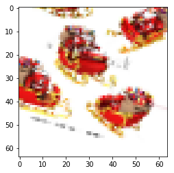
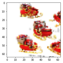
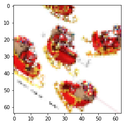
ImageDataGenerator becomes really useful when we actually want to generate more data. We'll show you how this works.
train_datagen= ImageDataGenerator(rescale=1./255,
     rotation_range=40,
     width_shift_range=0.2,
     height_shift_range=0.2,
     shear_range=0.3,
     zoom_range=0.1,
     horizontal_flip = False)
names = [os.path.join(train_santa, name) for name in os.listdir(train_santa)]
img_path = names[91]
img = load_img(img_path, target_size=(64, 64))
reshape_img = img_to_array(img)
reshape_img = reshape_img.reshape((1,) + reshape_img.shape)
i=0
for batch in train_datagen.flow(reshape_img, batch_size=1):
plt.figure(i)
imgplot = plt.imshow(array_to_img(batch[0]))
i += 1
if i % 3 == 0:
break
plt.show()# get all the data in the directory split/test (180 images), and reshape them
test_generator = ImageDataGenerator(rescale=1./255).flow_from_directory(
test_folder,
target_size=(64, 64),
batch_size = 180,
class_mode='binary')
# get all the data in the directory split/validation (200 images), and reshape them
val_generator = ImageDataGenerator(rescale=1./255).flow_from_directory(
val_folder,
target_size=(64, 64),
batch_size = 32,
class_mode='binary')
# get all the data in the directory split/train (542 images), and reshape them
train_generator = train_datagen.flow_from_directory(
train_folder,
target_size=(64, 64),
batch_size = 32,
class_mode='binary')Found 180 images belonging to 2 classes.
Found 200 images belonging to 2 classes.
Found 542 images belonging to 2 classes.
model = models.Sequential()
model.add(layers.Conv2D(32, (3, 3), activation='relu',
                        input_shape=(64 ,64,  3)))
model.add(layers.MaxPooling2D((2, 2)))

model.add(layers.Conv2D(32, (4, 4), activation='relu'))
model.add(layers.MaxPooling2D((2, 2)))

model.add(layers.Conv2D(64, (3, 3), activation='relu'))
model.add(layers.MaxPooling2D((2, 2)))

model.add(layers.Flatten())
model.add(layers.Dense(64, activation='relu'))
model.add(layers.Dense(1, activation='sigmoid'))

model.compile(loss='binary_crossentropy',
              optimizer= 'sgd',
              metrics=['acc'])
history_2 = model.fit_generator(
train_generator,
steps_per_epoch=25,
epochs=30,
validation_data=val_generator,
validation_steps=25)Epoch 1/30
25/25 [==============================] - 24s 959ms/step - loss: 0.6825 - acc: 0.5088 - val_loss: 0.6784 - val_acc: 0.4931
Epoch 2/30
25/25 [==============================] - 18s 731ms/step - loss: 0.6809 - acc: 0.4889 - val_loss: 0.6705 - val_acc: 0.5057
Epoch 3/30
25/25 [==============================] - 19s 759ms/step - loss: 0.6700 - acc: 0.5099 - val_loss: 0.6649 - val_acc: 0.4986
Epoch 4/30
25/25 [==============================] - 19s 756ms/step - loss: 0.6716 - acc: 0.4925 - val_loss: 0.6545 - val_acc: 0.5142
Epoch 5/30
25/25 [==============================] - 18s 720ms/step - loss: 0.6618 - acc: 0.4953 - val_loss: 0.6480 - val_acc: 0.5412
Epoch 6/30
25/25 [==============================] - 17s 692ms/step - loss: 0.6488 - acc: 0.5585 - val_loss: 0.6350 - val_acc: 0.5426
Epoch 7/30
25/25 [==============================] - 17s 698ms/step - loss: 0.6406 - acc: 0.5986 - val_loss: 0.6131 - val_acc: 0.6179
Epoch 8/30
25/25 [==============================] - 18s 703ms/step - loss: 0.6182 - acc: 0.6848 - val_loss: 0.5917 - val_acc: 0.5701
Epoch 9/30
25/25 [==============================] - 19s 747ms/step - loss: 0.5995 - acc: 0.7053 - val_loss: 0.5610 - val_acc: 0.7159
Epoch 10/30
25/25 [==============================] - 19s 778ms/step - loss: 0.5746 - acc: 0.7722 - val_loss: 0.5229 - val_acc: 0.8736
Epoch 11/30
25/25 [==============================] - 21s 820ms/step - loss: 0.5355 - acc: 0.8202 - val_loss: 0.4920 - val_acc: 0.7500
Epoch 12/30
25/25 [==============================] - 18s 716ms/step - loss: 0.5157 - acc: 0.7957 - val_loss: 0.4750 - val_acc: 0.8558
Epoch 13/30
25/25 [==============================] - 19s 753ms/step - loss: 0.5224 - acc: 0.7517 - val_loss: 0.4509 - val_acc: 0.8679
Epoch 14/30
25/25 [==============================] - 17s 695ms/step - loss: 0.4365 - acc: 0.8322 - val_loss: 0.4074 - val_acc: 0.8608
Epoch 15/30
25/25 [==============================] - 19s 751ms/step - loss: 0.4558 - acc: 0.7927 - val_loss: 0.3604 - val_acc: 0.8626
Epoch 16/30
25/25 [==============================] - 15s 619ms/step - loss: 0.3974 - acc: 0.8244 - val_loss: 0.6614 - val_acc: 0.6222
Epoch 17/30
25/25 [==============================] - 18s 703ms/step - loss: 0.3881 - acc: 0.8430 - val_loss: 0.4041 - val_acc: 0.7926
Epoch 18/30
25/25 [==============================] - 18s 707ms/step - loss: 0.3873 - acc: 0.8208 - val_loss: 0.2955 - val_acc: 0.8991
Epoch 19/30
25/25 [==============================] - 20s 793ms/step - loss: 0.3690 - acc: 0.8472 - val_loss: 0.5001 - val_acc: 0.7418
Epoch 20/30
25/25 [==============================] - 19s 767ms/step - loss: 0.3411 - acc: 0.8567 - val_loss: 0.3544 - val_acc: 0.8693
Epoch 21/30
25/25 [==============================] - 17s 682ms/step - loss: 0.3096 - acc: 0.8796 - val_loss: 0.2478 - val_acc: 0.9190
Epoch 22/30
25/25 [==============================] - 18s 724ms/step - loss: 0.2971 - acc: 0.8921 - val_loss: 0.2591 - val_acc: 0.9217
Epoch 23/30
25/25 [==============================] - 17s 700ms/step - loss: 0.2797 - acc: 0.8945 - val_loss: 0.2508 - val_acc: 0.8963
Epoch 24/30
25/25 [==============================] - 17s 694ms/step - loss: 0.3001 - acc: 0.8614 - val_loss: 0.3669 - val_acc: 0.8585
Epoch 25/30
25/25 [==============================] - 19s 751ms/step - loss: 0.2836 - acc: 0.8869 - val_loss: 0.2718 - val_acc: 0.9233
Epoch 26/30
25/25 [==============================] - 19s 745ms/step - loss: 0.2654 - acc: 0.9030 - val_loss: 0.2096 - val_acc: 0.9272
Epoch 27/30
25/25 [==============================] - 16s 645ms/step - loss: 0.2532 - acc: 0.8948 - val_loss: 0.2557 - val_acc: 0.9176
Epoch 28/30
25/25 [==============================] - 17s 690ms/step - loss: 0.2838 - acc: 0.8935 - val_loss: 0.2240 - val_acc: 0.9261
Epoch 29/30
25/25 [==============================] - 18s 728ms/step - loss: 0.2906 - acc: 0.8950 - val_loss: 0.2873 - val_acc: 0.8984
Epoch 30/30
25/25 [==============================] - 24s 970ms/step - loss: 0.2447 - acc: 0.9083 - val_loss: 0.2566 - val_acc: 0.9048
test_x, test_y = next(test_generator)results_test = model.evaluate(test_x, test_y)180/180 [==============================] - 0s 1ms/step
results_test[0.2512160725063748, 0.9277777751286824]
In this code along lab, we looked again at some of the preprocessing techniques needed in order to organize our data prior to building a model using Keras. Afterwards, we investigated new code in order to build a CNN for image recognition.


