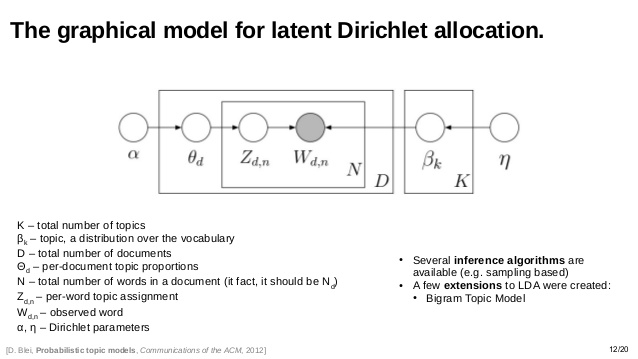
This is a collection documenting the resources I find related to topic models with an R flavored focus. A topic model is a type of generative model used to "discover" latent topics that compose a corpus or collection of documents. Typically topic modeling is used on a collection of text documents but can be used for other modes including use as caption generation for images.
- Just the Essentials
- Key Players
- Videos
- Articles
- Websites & Blogs
- R Resources
- Topic Modeling R Demo
- Contributing
This is my run down of the minimal readings, websites, videos, & scripts the reader needs to become familiar with topic modeling. The list is in an order I believe will be of greatest use and contains a nice mix of introduction, theory, application, and interpretation. As you want to learn more about topic modeling, the other sections will become more useful.
- Boyd-Graber, J. (2013). Computational Linguistics I: Topic Modeling
- Underwood, T. (2012). Topic Modeling Made Just Simple Enough
- Weingart, S. (2012). Topic Modeling for Humanists: A Guided Tour
- Blei, D. M. (2012). Probabilistic topic models. *Communications of the ACM, (55)*4, 77-84. doi:10.1145/2133806.2133826
- inkhorn82 (2014). A Delicious Analysis! (aka topic modelling using recipes) (CODE)
- Grüen, B. & Hornik, K. (2011). topicmodels: An R Package for Fitting Topic Models.. Journal of Statistical Software, 40(13), 1-30.
- Marwick, B. (2014a). The input parameters for using latent Dirichlet allocation
- Tang, J., Meng, Z., Nguyen, X. , Mei, Q. , & Zhang, M. (2014). Understanding the limiting factors of topic modeling via posterior contraction analysis. In 31 st International Conference on Machine Learning, 190-198.
- Sievert, C. (2014). LDAvis: A method for visualizing and interpreting topic models
- Rhody, L. M. (2012). Some Assembly Required: Understanding and Interpreting Topics in LDA Models of Figurative Language
- Rinker, T.W. (2015). R Script: Example Topic Model Analysis
Papadimitriou, Raghavan, Tamaki & Vempala, Santosh (1997) first introduced the notion of topic modeling in their "Latent Semantic Indexing: A probabilistic analysis". Thomas Hofmann (1999) developed "Probabilistic latent semantic indexing". Blei, Ng, & Jordan (2003) proposed latent Dirichlet allocation (LDA) as a means of modeling documents with multiple topics but assumes the topic are uncorrelated. Blei & Lafferty (2007) proposed correlated topics model (CTM), extending LDA to allow for correlations between topics. Roberts, Stewart, Tingley, & Airoldi (2013) propose a Structural Topic Model (STM), allowing the inclusion of meta-data in the modeling process.
- Boyd-Graber, J. (2013). Computational Linguistics I: Topic Modeling
- Blei, D. (2007) Modeling Science: Dynamic Topic Models of Scholarly Research
- Blei, D. (2009) Topic Models: Parts I & II (Lecture Notes)
- Jordan, M. (2014) A Short History of Topic Models
- Sievert, C. (2014) LDAvis: A method for visualizing and interpreting topic models
- Maybe, B. (2015) SavvySharpa: Visualizing Topic Models
-
Marwick, B. 2013. Discovery of Emergent Issues and Controversies in Anthropology Using Text Mining, Topic Modeling, and Social Network Analysis of Microblog Content. In Yanchang Zhao, Yonghua Cen (eds) Data Mining Applications with R. Elsevier. p. 63-93
-
Newman, D.J. & Block, S. (2006). Probabilistic topic decomposition of an eighteenth-century American newspaper. Journal of the American Society for Information Science and Technology. 57(6), 753-767. doi:10.1002/asi.v57:6
- Blei, D. M. (2012). Probabilistic topic models. *Communications of the ACM, (55)*4, 77-84. doi:10.1145/2133806.2133826
- Blei, D. M. & Lafferty, J. D. (2007) A correlated topic model of Science. The Annals of Applied Statistics 1(1), 17-35. doi:10.1214/07-AOAS114
- Blei, D. M. & Lafferty, J. D. (2009) Topic models. In A Srivastava, M Sahami (eds.), Text mining: classification, clustering, and applications. Chapman & Hall/CRC Press. 71-93.
- Blei, D. M. & McAuliffe, J. (2008). Supervised topic models. In Advances in Neural Information Processing Systems 20, 1-8.
- Blei, D. M., Ng, A.Y., & Jordan, M.I. (2003). Latent Dirichlet Allocation. Journal of Machine Learning Research, 3, 993-1022.
- Chang, J., Boyd-Graber, J. , Wang, C., Gerrish, S., & Blei. D. (2009). Reading tea leaves: How humans interpret topic models. In Neural Information Processing Systems.
- Griffiths, T.L. & Steyvers, M. (2004). Finding Scientific Topics. Proceedings of the National Academy of Sciences of the United States of America, 101, 5228-5235.
- Griffiths, T.L., Steyvers, M., & Tenenbaum, J.B.T. (2007). Topics in Semantic Representation. Psychological Review, 114(2), 211-244.
- Grüen, B. & Hornik, K. (2011). topicmodels: An R Package for Fitting Topic Models.. Journal of Statistical Software, 40(13), 1-30.
- Mimno, D. & A. Mccallum. (2007). Organizing the OCA: learning faceted subjects from a library of digital books. In Joint Conference on Digital Libraries. ACM Press, New York, NY, 376–385.
- Ponweiser, M. (2012). Latent Dirichlet Allocation in R (Diploma Thesis). Vienna University of Economics and Business, Vienna
- Roberts M.E., Stewart B.M., Tingley D., & Airoldi E.M. (2013) The Structural Topic Model and Applied Social Science. Advances in Neural Information Processing Systems Workshop on Topic Models: Computation, Application, and Evaluation, 1-4.
- Roberts, M., Stewart, B., Tingley, D., Lucas, C., Leder-Luis, J., Gadarian, S., Albertson, B., et al. (2014). Structural topic models for open ended survey responses. American Journal of Political Science, American Journal of Political Science, 58(4), 1064-1082.
- Roberts, M., Stewart, B., Tingley, D. (n.d.). stm: R Package for Structural Topic Models, 1-49.
- Sievert, C. & Shirley, K. E. (2014a). LDAvis: A Method for Visualizing and Interpreting Topics. in Proceedings of the Workshop on Interactive Language Learning, Visualization, and Interfaces 63-70.
- Steyvers, M. & Griffiths, T. (2007). Probabilistic topic models. In T. Landauer, D McNamara, S. Dennis, and W. Kintsch (eds), Latent Semantic Analysis: A Road to Meaning. Laurence Erlbaum
- Taddy, M.A. (2012). On Estimation and Selection for Topic Models In Proceedings of the 15th International Conference on Artificial Intelligence and Statistics (AISTATS 2012), 1184-1193.
- Tang, J., Meng, Z., Nguyen, X. , Mei, Q. , & Zhang, M. (2014). Understanding the limiting factors of topic modeling via posterior contraction analysis. In 31 st International Conference on Machine Learning, 190-198.
- Blei, D. (n.d.). Topic Modeling
- Jockers, M.L. (2013). "Secret" Recipe for Topic Modeling Themes
- Jones, T. (n.d.). Topic Models Reading List
- Marwick, B. (2014a). The input parameters for using latent Dirichlet allocation
- Marwick, B. (2014b). Topic models: cross validation with loglikelihood or perplexity
- Rhody, L. M. (2012). Some Assembly Required: Understanding and Interpreting Topics in LDA Models of Figurative Language
- Schmidt, B.M. (2012). Words Alone: Dismantling Topic Models in the Humanities
- Underwood, T. (2012a). Topic Modeling Made Just Simple Enough
- Underwood, T. (2012b). What kinds of "topics" does topic modeling actually produce?
- Weingart, S. (2012). Topic Modeling for Humanists: A Guided Tour
- Weingart, S. (2011). Topic Modeling and Network Analysis
| Package | Functionality | Pluses | Author | R Language Interface |
|---|---|---|---|---|
| lda* | Collapsed Gibbs for LDA | Graphing utilities | Chang | R |
| topicmodels | LDA and CTM | Follows Blei's implementation; great vignette; takes | C | DTM |
| stm | Model w/ meta-data | Great documentation; nice visualization | Roberts, Stewart, & Tingley | C |
| LDAvis | Interactive visualization | Aids in model interpretation | Sievert & Shirley | R + Shiny |
| mallet** | LDA | MALLET is well known | Mimno | Java |
*StackExchange discussion of lda vs.
topicmodels
**Setting Up
MALLET
- Chang J. (2010). lda: Collapsed Gibbs Sampling Methods for Topic Models. http://CRAN.R-project.org/package=lda.
- Grüen, B. & Hornik, K. (2011). topicmodels: An R Package for Fitting Topic Models.. Journal of Statistical Software, 40(13), 1-30.
- Mimno, D. (2013). vignette-mallet: A wrapper around the Java machine learning tool MALLET. https://CRAN.R-project.org/package=mallet
- Ponweiser, M. (2012). Latent Dirichlet Allocation in R (Diploma Thesis). Vienna University of Economics and Business, Vienna.
- Roberts, M., Stewart, B., Tingley, D. (n.d.). stm: R Package for Structural Topic Models, 1-49.
- Sievert, C. & Shirley, K. E. (2014a). LDAvis: A Method for Visualizing and Interpreting Topics. Proceedings of the Workshop on Interactive Language Learning, Visualization, and Interfaces 63-70.
- Sievert, C. & Shirley, K. E. (2014b). Vignette: LDAvis details. 1-5.
- Awati, K. (2015). A gentle introduction to topic modeling using R
- Dubins, M. (2013). Topic Modeling in Python and R: A Rather Nosy Analysis of the Enron Email Corpus
- Goodrich, B. (2015) Topic Modeling Twitter Using R (CODE)
- inkhorn82 (2014). A Delicious Analysis! (aka topic modelling using recipes) (CODE)
- Jockers, M.L. (2014).Introduction to Text Analysis and Topic Modeling with R
- Medina, L. (2015). Conspiracy Theories - Topic Modeling & Keyword Extraction
- Sievert, C. (n.d.). A topic model for movie reviews
- Sievert, C. (2014). Topic Modeling In R
The .R script for this demonstration can be downloaded from scripts/Example_topic_model_analysis.R
if (!require("pacman")) install.packages("pacman")
pacman::p_load_gh("trinker/gofastr")
pacman::p_load(tm, topicmodels, dplyr, tidyr, igraph, devtools, LDAvis, ggplot2)

## Source topicmodels2LDAvis & optimal_k functions
invisible(lapply(
    file.path(
        "https://raw.githubusercontent.com/trinker/topicmodels_learning/master/functions",
        c("topicmodels2LDAvis.R", "optimal_k.R")
    ),
    devtools::source_url
))

## SHA-1 hash of file is 5ac52af21ce36dfe8f529b4fe77568ced9307cf0
## SHA-1 hash of file is 7f0ab64a94948c8b60ba29dddf799e3f6c423435

data(presidential_debates_2012)
stops <- c(
        tm::stopwords("english"),
        tm::stopwords("SMART"),
        "governor", "president", "mister", "obama","romney"
    ) %>%
    gofastr::prep_stopwords()
doc_term_mat <- presidential_debates_2012 %>%
    with(gofastr::q_dtm_stem(dialogue, paste(person, time, sep = "_"))) %>%
    gofastr::remove_stopwords(stops, stem=TRUE) %>%
    gofastr::filter_tf_idf() %>%
    gofastr::filter_documents()
control <- list(burnin = 500, iter = 1000, keep = 100, seed = 2500)
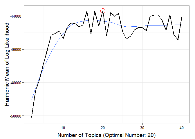
The plot below shows the harmonic mean of the log likelihoods against k (number of topics).
(k <- optimal_k(doc_term_mat, 40, control = control))

##
## Grab a cup of coffee this could take a while...

## 10 of 40 iterations (Current: 08:54:32; Elapsed: .2 mins)
## 20 of 40 iterations (Current: 08:55:07; Elapsed: .8 mins; Remaining: ~2.3 mins)
## 30 of 40 iterations (Current: 08:56:03; Elapsed: 1.7 mins; Remaining: ~1.3 mins)
## 40 of 40 iterations (Current: 08:57:30; Elapsed: 3.2 mins; Remaining: ~0 mins)
## Optimal number of topics = 20
It appears the optimal number of topics is ~k = 20.
control[["seed"]] <- 100
lda_model <- topicmodels::LDA(doc_term_mat, k=as.numeric(k), method = "Gibbs",
    control = control)
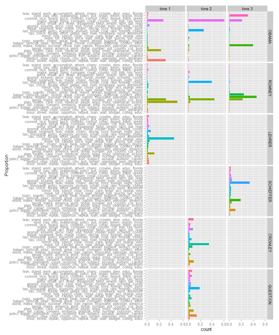
topics <- topicmodels::posterior(lda_model, doc_term_mat)[["topics"]]
topic_dat <- dplyr::add_rownames(as.data.frame(topics), "Person_Time")
colnames(topic_dat)[-1] <- apply(terms(lda_model, 10), 2, paste, collapse = ", ")

tidyr::gather(topic_dat, Topic, Proportion, -c(Person_Time)) %>%
    tidyr::separate(Person_Time, c("Person", "Time"), sep = "_") %>%
    dplyr::mutate(Person = factor(Person,
        levels = c("OBAMA", "ROMNEY", "LEHRER", "SCHIEFFER", "CROWLEY", "QUESTION" ))
    ) %>%
    ggplot2::ggplot(ggplot2::aes(weight=Proportion, x=Topic, fill=Topic)) +
        ggplot2::geom_bar() +
        ggplot2::coord_flip() +
        ggplot2::facet_grid(Person~Time) +
        ggplot2::guides(fill=FALSE) +
        ggplot2::xlab("Proportion")
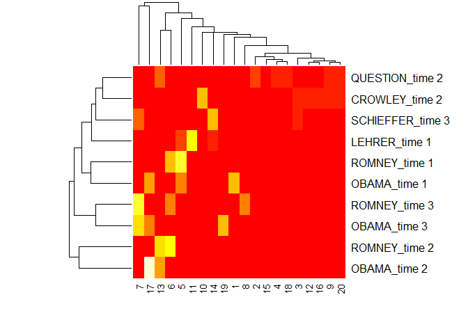
heatmap(topics, scale = "none")
post <- topicmodels::posterior(lda_model)

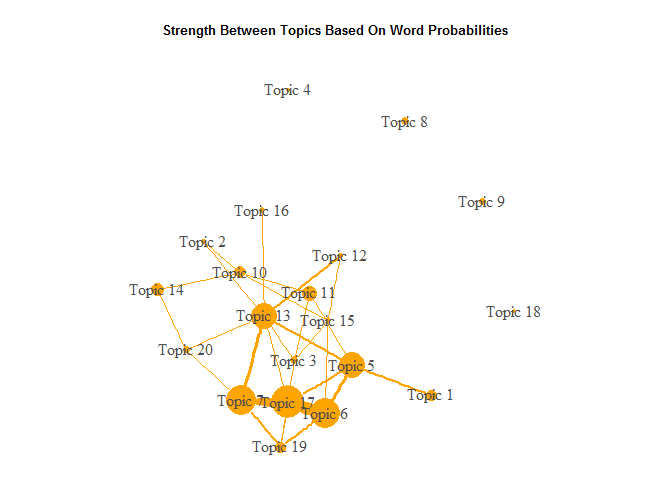
cor_mat <- cor(t(post[["terms"]]))
cor_mat[ cor_mat < .05 ] <- 0
diag(cor_mat) <- 0

graph <- graph.adjacency(cor_mat, weighted=TRUE, mode="lower")
graph <- delete.edges(graph, E(graph)[ weight < 0.05])

E(graph)$edge.width <- E(graph)$weight*20
V(graph)$label <- paste("Topic", V(graph))
V(graph)$size <- colSums(post[["topics"]]) * 15

par(mar=c(0, 0, 3, 0))
set.seed(110)
plot.igraph(graph, edge.width = E(graph)$edge.width,
    edge.color = "orange", vertex.color = "orange",
    vertex.frame.color = NA, vertex.label.color = "grey30")
title("Strength Between Topics Based On Word Probabilities", cex.main=.8)
minval <- .1
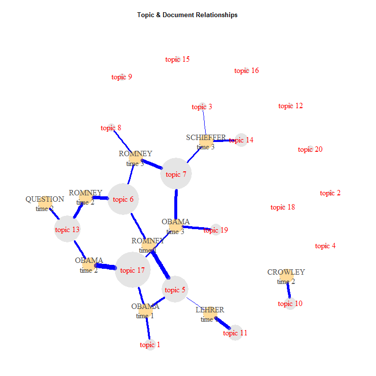
topic_mat <- topicmodels::posterior(lda_model)[["topics"]]

graph <- graph_from_incidence_matrix(topic_mat, weighted=TRUE)
graph <- delete.edges(graph, E(graph)[ weight < minval])

E(graph)$edge.width <- E(graph)$weight*17
E(graph)$color <- "blue"
V(graph)$color <- ifelse(grepl("^\\d+$", V(graph)$name), "grey75", "orange")
V(graph)$frame.color <- NA
V(graph)$label <- ifelse(grepl("^\\d+$", V(graph)$name), paste("topic", V(graph)$name), gsub("_", "\n", V(graph)$name))
V(graph)$size <- c(rep(10, nrow(topic_mat)), colSums(topic_mat) * 20)
V(graph)$label.color <- ifelse(grepl("^\\d+$", V(graph)$name), "red", "grey30")

par(mar=c(0, 0, 3, 0))
set.seed(369)
plot.igraph(graph, edge.width = E(graph)$edge.width,
    vertex.color = adjustcolor(V(graph)$color, alpha.f = .4))
title("Topic & Document Relationships", cex.main=.8)
The output from LDAvis is not easily embedded within an R markdown document, however, the reader may see the results here.
lda_model %>%
    topicmodels2LDAvis() %>%
    LDAvis::serVis()
## Create the DocumentTermMatrix for New Data
doc_term_mat2 <- partial_republican_debates_2015 %>%
    with(gofastr::q_dtm_stem(dialogue, paste(person, location, sep = "_"))) %>%
    gofastr::remove_stopwords(stops, stem=TRUE) %>%
    gofastr::filter_tf_idf() %>%
    gofastr::filter_documents()


## Update Control List
control2 <- control
control2[["estimate.beta"]] <- FALSE


## Run the Model for New Data
lda_model2 <- topicmodels::LDA(doc_term_mat2, k = k, model = lda_model,
    control = list(seed = 100, estimate.beta = FALSE))


## Plot the Topics Per Person & Location for New Data
topics2 <- topicmodels::posterior(lda_model2, doc_term_mat2)[["topics"]]
topic_dat2 <- dplyr::add_rownames(as.data.frame(topics2), "Person_Location")
colnames(topic_dat2)[-1] <- apply(terms(lda_model2, 10), 2, paste, collapse = ", ")

tidyr::gather(topic_dat2, Topic, Proportion, -c(Person_Location)) %>%
    tidyr::separate(Person_Location, c("Person", "Location"), sep = "_") %>%
    ggplot2::ggplot(ggplot2::aes(weight=Proportion, x=Topic, fill=Topic)) +
        ggplot2::geom_bar() +
        ggplot2::coord_flip() +
        ggplot2::facet_grid(Person~Location) +
        ggplot2::guides(fill=FALSE) +
        ggplot2::xlab("Proportion")


## LDAvis of Model for New Data
lda_model2 %>%
    topicmodels2LDAvis() %>%
    LDAvis::serVis()
You are welcome to:
- submit suggestions and bug-reports at: https://github.com/trinker/topicmodels_learning/issues
- send a pull request on: https://github.com/trinker/topicmodels_learning/
- compose a friendly e-mail to: tyler.rinker@gmail.com

