Mostafa-M-Rezaee/water-forecast

Machine learning models applied to water demand forecasting in the City of London.

Water Demand Forecasting

The purpose of this project is to deliver a machine learning solution to forecasting aggregate water demand. This work was led by the Municipal Artificial Intelligence Applications Lab out of the Information Technology Services division. This repository contains the code used to fit multiple types of machine learning models to predict future daily water consumption. This repository is intended to serve as an example for other municipalities who wish to explore water demand forecasting in their own locales.

Table of Contents

1. Getting Started
2. Use Cases
   i) Train a model and visualize forecasts
   ii) Train all models
   iii) Bayesian hyperparameter optimization
   iv) Forecasting with a trained model
   v) Cross validation
   vi) Client clustering experiment (using K-Prototypes)
   vii) Model interpretability
3. Data Preprocessing
4. Troubleshooting
5. Project Structure
6. Project Config
7. Azure Machine Learning Pipelines
8. Contact

Getting Started

1. Clone this repository (for help see this tutorial).
2. Install the necessary dependencies (listed in requirements.txt). To do this, open a terminal in the root directory of the project and run the following:

   $ pip install -r requirements.txt
   

3. Obtain raw water consumption data and preprocess it accordingly. See Data preprocessing for more details.
4. Update the TRAIN >> MODEL field of config.yml with the appropriate string representing the model type you wish to train. To train a model, ensure the TRAIN >> EXPERIMENT field is set to 'train_single'.
5. Execute train.py to train your chosen model on your preprocessed data. The trained model will be serialized within results/models/, and its filename will resemble the following structure: {modeltype}{yyyymmdd-hhmmss}.{ext}, where {modeltype} is the type of model trained, {yyyymmdd-hhmmss} is the current time, and {ext} is the appropriate file extension.
6. Navigate to results/experiments/ to see the performance metrics achieved by the model's forecast on the test set. The file name will be {modeltype}eval{yyyymmdd-hhmmss}.csv. You can find a visualization of the test set forecast in img/forecast_visualizations/. Its filename will be {modeltype}forecast{yyyymmdd-hhmmss}.png.

Use Cases

Train a model and visualize a forecast

1. Once you have obtained a preprocessed dataset (see step 3 of Getting Started, ensure that the preprocessed dataset is located in data/preprocessed/ with filename "preprocessed_data.csv".
2. In config.yml, set EXPERIMENT >> TRAIN to 'single_train'. Set TRAIN >> MODEL to the appropriate string representing the model type you wish to train.
3. Execute train.py to train your chosen model on your preprocessed data. The trained model will be serialized within results/models/, and its filename will resemble the following structure: {modeltype}{yyyymmdd-hhmmss}.{ext}, where {modeltype} is the type of model trained, {yyyymmdd-hhmmss} is the current time, and {ext} is the appropriate file extension.
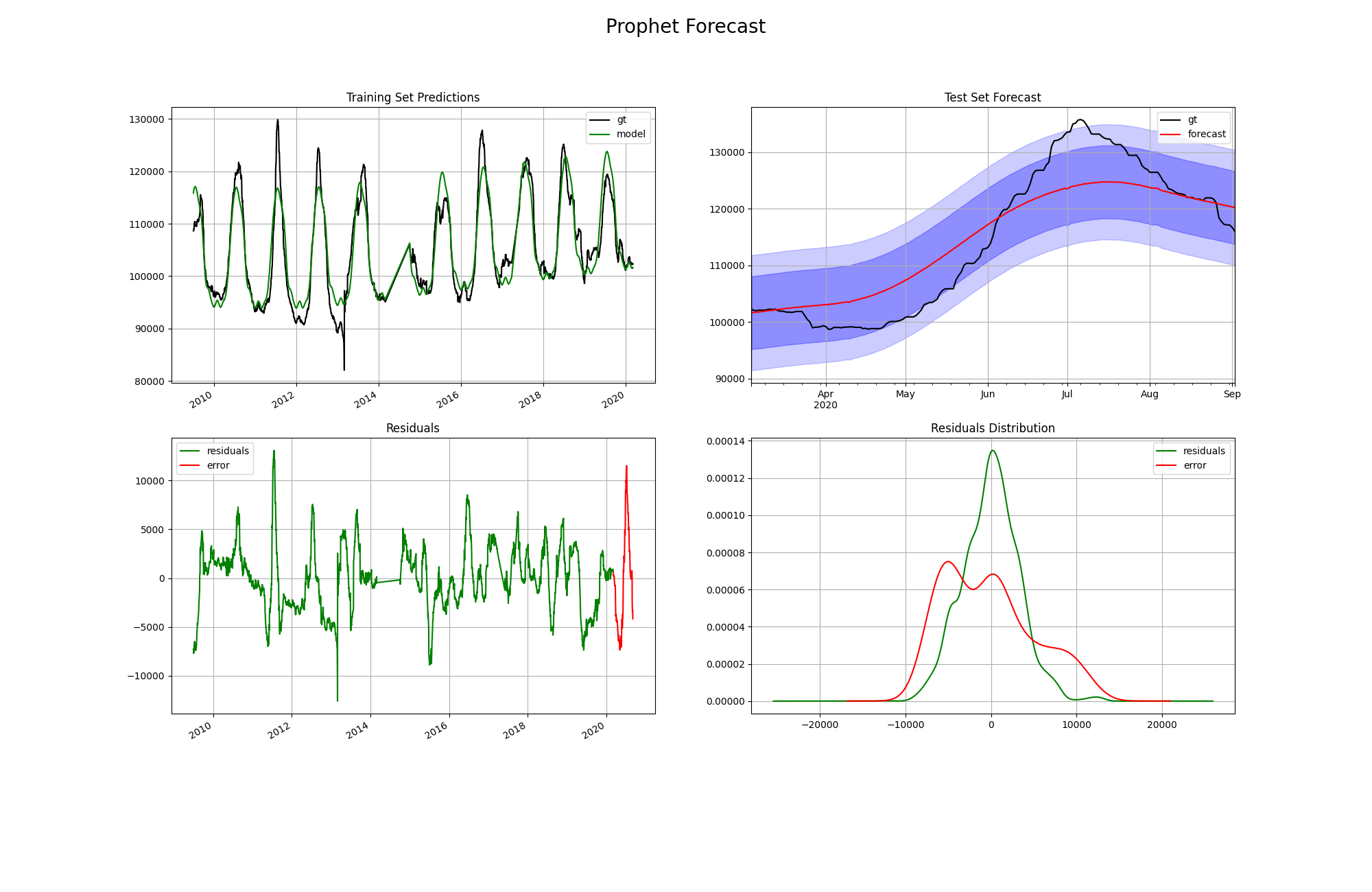
4. Navigate to results/experiments/ to see the performance metrics achieved by the model's forecast on the test set. The file name will be {modeltype}eval{yyyymmdd-hhmmss}.csv. You can find a visualization of the test set forecast in img/forecast_visualizations/. Its filename will be {modeltype}forecast{yyyymmdd-hhmmss}.png. This visualization displays training set predictions, test set forecasts, test set predictions (depending on the model type), training residuals, and test error. The image below is an example of one of a test set forecast visualization.

Train all models

We investigated several different model types for the task of water demand forecasting. As such, we followed the Strategy Design Pattern to encourage rapid prototyping of our models. This pattern allows the user to interact with models using a common interface to perform core operations in the machine learning workflow (e.g. train, forecast, serialize the model). We investigated the following models:

• Prophet
• Recurrent neural network with LSTM layer
• Recurrent neural network with GRU layer
• Convolutional neural network with 1D convolutional layers
• ARIMA
• SARIMAX
• Ordinary least-squares linear regression
• Random forest regression

The following steps describe how to train all models.

1. Once you have obtained a preprocessed dataset (see step 3 of Getting Started, ensure that the preprocessed dataset is located in data/preprocessed/ with filename "preprocessed_data.csv".
2. In config.yml, set EXPERIMENT >> TRAIN to 'all_train'.
3. Execute train.py to train each model on your preprocessed data. Performance metrics and test set forecast visualizations will be saved for each model, as described in Step 4 of Train a model and visualize a forecast.

Bayesian hyperparameter optimization

Hyperparameter optimization is an important part of the standard machine learning workflow. We chose to conduct Bayesian hyperparameter optimization. The results of the optimization informed the final hyperparameters currently set in the HPARAMS sections of config.yml. The objective of the Bayesian optimization was the minimization of mean absolute error in the average test set forecast resulting from a time series cross validation. With the help of the scikit-optimize package, we were able to visualize the effects of single hyperparameters and pairs of hyperparameters on the objective.

To conduct your own Bayesian hyperparameter optimization, you may follow the steps below. Note that if you are not planning on changing the default hyperparameter ranges set in the HPARAM_SEARCH section of config.yml, you may skip step 2.

1. In config.yml, set EXPERIMENT >> TRAIN to 'hparam_search'. Set TRAIN >> MODEL to the appropriate string representing the model type you wish to train.
2. In the TRAIN >> HPARAM_SEARCH >> MAX_EVALS field of config.yml, set the maximum number of combinations of hyperparameters to test. In the TRAIN >> HPARAM_SEARCH >> LAST_FOLDS field, set the number of folds from cross validation to average the test set forecast objective over. If you wish to change the objective metric, update TRAIN >> HPARAM_SEARCH >> HPARAM_OBJECTIVE accordingly.
3. Set the ranges of hyperparameters you wish to study in the HPARAM_SEARCH >> {MODEL} subsection of config.yml, where {{MODEL}} is the model name you set in Step 1. The config file already has a comprehensive set of hyperparameter ranges defined for each model type, so you may not need to change anything in this step. Consider whether your hyperparameter ranges are sets, integer ranges, or float ranges, and whether they need to be investigated on a uniform or logarithmic range. See below for an example of how to correctly set ranges for different types of hyperparameters.

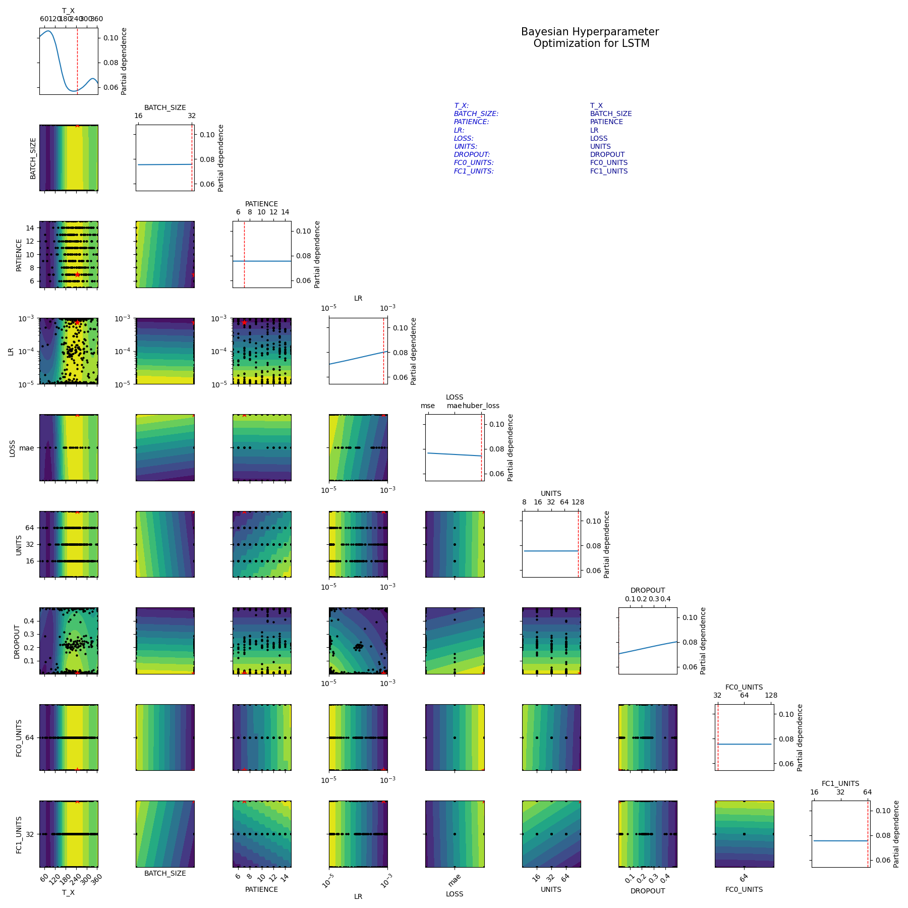
    FC0_UNITS:
      TYPE: 'set'
      RANGE: [32, 64, 128]
    DROPOUT:
      TYPE: 'float_uniform'
      RANGE: [0.0, 0.5]
    LR:
      TYPE: 'float_log'
      RANGE: [0.00001, 0.001]   
    PATIENCE:
      TYPE: 'int_uniform'
      RANGE: [5, 15]      
   

4. Execute train.py. A CSV log detailing the trials in the Bayesian optimization will be located in results/experiments/hparam_search_{modelname}_{yyyymmdd-hhmmss}.csv, where {modeltype} is the type of model investigated, and {yyyymmdd-hhmmss} is the current time. Each row in the CSV will detail the hyperparameters used for a particular trial, along with the value of the objective from the cross validation run with those hyperparameters. The final row details the best trial, which contains the optimal hyperparameter values. The visualization of the search can be found at img/experiment_visualizations/Bayesian_opt_{modeltype}_{yyyymmdd-hhmmss}.png. See below for an example of a Bayesian hyperparameter optimization visualization for an LSTM-based model. For details on how to interpret this visualization, see this entry in the scikit-optimize docs.

Forecasting with a trained model

Once a model has been fitted, the user may wish to obtain water consumption forecasts for future dates. Note that forecasts differ from predictions in that each prediction may be used in part to make a prediction for the next day. To obtain predictions for any number of days following the final date in the training set, follow the steps below.

1. Ensure that you have already trained a model (see Train a model and visualize a forecast).
2. In config.yml, set FORECAST >> MODEL to the type of model you trained. Set FORECAST >> MODEL_PATH to the path of the serialization of the model. Set FORECAST >> DAYS to the number of future days you wish to make forecasts for.
3. Execute src/predict.py. The model will be loaded from disk and will generate a forecast for the desired number of days.
4. A CSV containing the forecast will be saved to 'results/predictions/forecast_{modelname}_{days}d_{yyyymmdd-hhmmss}.csv, where {modeltype} is the type of model investigated, {days} is the length of the forecast in days, and {yyyymmdd-hhmmss} is the current time.

Prophet Forecast Visualization

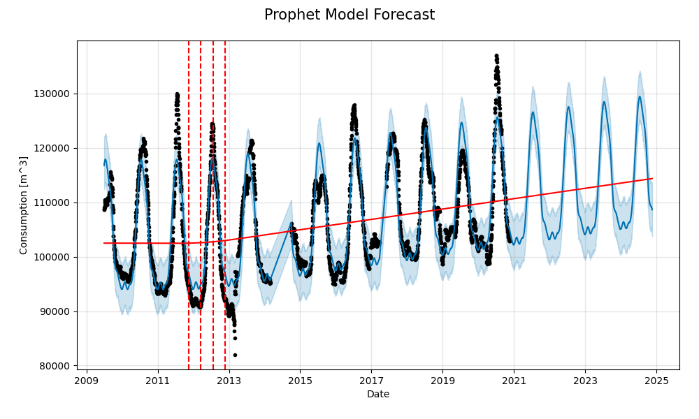
If you have loaded a Prophet model for forecasting, you may use the Prophet package to produce a visualization of the forecast, complete with uncertainty intervals. This is done automatically when executing a train experiment using a Prophet model. Alternatively, add a call to plot_prophet_forecast(prophet_model, prophet_pred) (implemented in visualize.py to the code. By default the image will be saved to 'img/forecast_visualizations/Prophet_API_forecast{yyyymmdd-hhmmss}.png. Below is an example of such an image, portraying a 4-year forecast.

Cross validation

Cross validation helps us select a model that is as unbiased as possible towards any particular dataset. By using cross validation, we can be increasingly confident in the generalizability of our model in the future. We employ a time series variant of k-fold cross validation to validate our model. First, we divide our dataset into a set of quantiles (e.g. 10 deciles). For the k^th split, the k^th quantile comprises the test set, and the training set is composed of all data preceding the k^th quantile. All data after the k^th quantile is disregarded for that particular fold. To run a cross validation experiment, follow the steps below.

1. Once you have obtained a preprocessed dataset (see step 3 of Getting Started, ensure that the preprocessed dataset is located in data/preprocessed/ with filename "preprocessed_data.csv".
2. In config.yml, set EXPERIMENT >> TRAIN to 'cross_validation'. Set TRAIN >> MODEL to the appropriate string representing the model type you wish to train. Set TRAIN >> N_QUANTILES to your chosen value for the number of quantiles to split the data into. Set TRAIN >> N_FOLDS to your chosen value for k.
3. Execute train.py to conduct cross validation with your chosen model. k models will be trained, each on successively larger datasets. A spreadsheet detailing test set forecast performance metrics for each of the k training experiments will be generated. The mean and standard deviation of each metric across the training experiments appear in the bottom 2 rows. Upon completion, it will be saved to 'results/predictions/cross_val_{modelname}_{yyyymmdd-hhmmss}.csv, where {modeltype} is the type of model trained and {yyyymmdd-hhmmss} is the current time.

Client clustering experiment (using K-Prototypes)

We were interested in investigating whether clients could be effectively clustered. We developed a separate preprocessing method that produced a feature vector for each client, including estimates of their monthly consumption over the past year, and other features pertaining to their water comsumption (e.g. meter type, land parcel area). Since our client feature vectors consisted of numerical and categorical data, and in the spirit of minimizing time complexity, k-prototypes was selected as the clustering algorithm. We wish to acknowledge Nico de Vos, as we made use of his implementation of k-prototypes. This experiment runs k-prototypes a series of times and selects the best clustering (i.e. least average dissimilarity between clients and their assigned clusters' centroids). Our intention was to provide city water management with an alternative means by which to categorize clients. The steps below detail how to cluster such a dataset.

1. Ensure that you have a CSV of client data saved to 'data/preprocessed/client_data.csv'. The primary key should be named CONTRACT_ACCOUNT. Ensure that the lists located in the DATA >> CATEGORICAL_FEATS and DATA >> BOOLEAN_FEATS fields of config.yml match the names of your categorical and boolean features respectively.
2. Set the EXPERIMENT field of the K-PROTOTYPES section of config.yml to 'cluster_clients'. Consult Project Config before changing the default values of oter parameters in config.yml.
3. Execute kprototypes.py.
4. 2 separate files will be saved once clustering is complete:
   1. A spreadsheet depicting cluster assignments by Contract Account number will be saved to results/experiments/client_clusters_{yyyymmdd-hhmmss}.csv, where {yyyymmdd-hhmmss} is the current time).
   2. Cluster centroids will be saved to a spreadsheet. Centroids have the same features as clients and their LIME explanations will be appended to the end by default. The spreadsheet will be saved to results/experiments/cluster_centroids_{yyyymmdd-hhmmss}.csv.

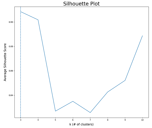
A tradeoff for the efficiency of k-prototypes is the fact that the number of clusters must be specified a priori. In an attempt to determine the optimal number of clusters, the Average Silhouette Method was implemented. During this procedure, different clusterings are computed for a range of values of k. A graph is produced that plots average Silhouette Score versus k. The higher average Silhouette Score is, the more optimal k is. To run this experiment, see the below steps.

1. Follow steps 1 and 2 as outlined above in the clustering instructions.
2. Set the K-PROTOTYPES >> EXPERIMENT field of config.yml to 'silhouette_analysis'. At this time, you may wish to change the K_MIN and K_MAX field of the K-PROTOTYPES section from their defaults. Values of k in the integer range of [K_MIN, K_MAX] will be investigated.
3. Execute kprototypes.py. An image depicting a graph of average Silhouette Score versus k will be saved to _img/data_visualizations/silhouette_plot_{yyyymmdd-hhmmss}.png. Upon visualizing this graph, note that a larger average Silhouette Score implies a better clustering. For example, in the below images, k = 3 is the best number of clusters.

Model interpretability

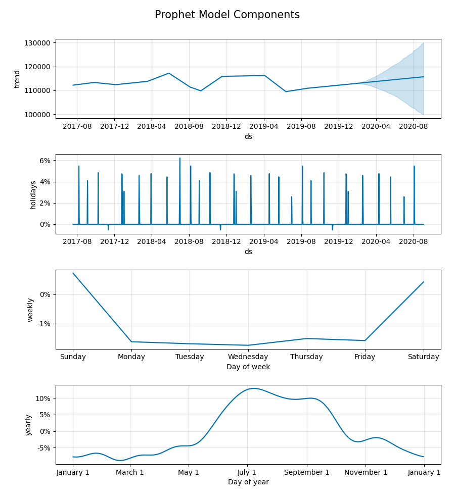
To gain insight into model functionality, we delved into the interpretability of our selected model. Currently, only the Prophet model is supported. The Prophet model is inherently interpretable, since it is a composition of interpretable functional components for trend, weekly periodicity, yearly periodicity, and holidays. The four components can be saved and plotted by following the below steps:

1. In config.yml, set TRAIN >> INTERPRETABILITY to true. Set TRAIN >> MODEL to 'prophet'.
2. Follow the steps in this document to run any training experiment (e.g. single train, train all, cross validation).
3. Upon completion of training, the values comprising the 4 components are saved to separate files in a new folder named results/interpretability/Prophet_{yyyymmdd-hhmmss}/, where {yyyymmdd-hhmmss} is the current datetime. The trend and holiday components are saved to CSV files detailing weights for each date. The weekly and yearly seasonality components are saved to JSON files containing their respective preiodic function parameters. A visualization of the components of the Prophet model can be found in img/interpretability_visualizations/Prophet_components_{yyyymmdd-hhmmss}.png. See below for an example of a visualization of the components of a Prophet model.

Data preprocessing

Our data preprocessing method is implemented in preprocess.py. Since water consumption database schemas vary considerably across jurisdictions, you likely will have to implement your own preprocessing script. The data that was used for our experiments was organized in a schema specific to London, Canada. Your preprocessed dataset should be a CSV file with at least the following columns:

• Date: A timestamp representing a date
• Consumption: A float representing an estimate of total water consumption on the date

Please see preprocessed_example.csv for an example of a preprocessed dataset containing the columns identified above. Many of the experiments described in this project's accompanying paper were conducted using this dataset.

Any other features you wish to use must have their own column. The model assumes all datatypes are numerical. As a result, categorical and Boolean features must be converted to a numeric representation. Below is a high-level overview of our preprocessing strategy.

Raw consumption data was provided to us as a set of CSV files containing consumption entries for each client at different billing periods. A single row consisted of a client's identifying information (e.g. contract account number), the start and end dates of their current billing period, how much water was consumed over the current billing period, and several other features pertaining to their water access (e.g. meter type, land parcel area, flags for certain billing considerations). In this repository, we included a sample of one such CSV file, with randomly inputted data, to demonstrate the features that we had available to us. These other features were numerical, categorical, or Boolean. Our goal was to transform all the raw data into a dataset that contained snapshots of the entire city's water consumption for each day. See the data dictionary for a complete categorization and description of the features that appeared in the CSV files comprising our raw data.

Aggregate system daily water consumption was estimated as follows. An estimate for each client's water consumption on a particular day was arrived at by dividing their water consumption over the billing period that the day fell under by the length of the billing period. We assumed uniform daily usage over the billing period because we did not have access to more granular data. The citywide estimate for water consumption on that day is then the sum of the daily estimates for each client.

Other features were aggregated to represent their state in the city as a whole for a particular day. Their value for each client was taken to be the value during the billing period including that day for that client. For each day, the average and standard deviation of numerical client features were taken to be daily estimates for that feature citywide. A similar approach was taken for Boolean features, whose values were 0 (false) or 1 (true) in raw data. The daily citywide estimate for that feature was the proportion of clients who had a value of "true" for that feature on that day. Citywide daily estimates of categorical client features were represented by a set of features for each value of the categorical feature, whereby each feature in the set represented the fraction of clients who had that value for that categorical feature. For example, each client had a feature categorizing the client as living in low, medium or high density residential regions. The preprocessed dataset had a feature for each of these values, indicating the fraction of clients living in low, medium or high density residential regions respectively on a given day.

We later discovered that the features other than consumption did not necessarily improve our forecasts. Thus, we abandoned the other features in our experiments, reducing our preprocessed dataset to a univariate dataset, mapping Date to Consumption. Note that some model architectures available in this repository require univariate data; when training these models, other features would be disregarded.

Troubleshooting

1. New raw data has a modified feature name

Data preprocessing issues can arise if a feature's name has been changed when providing a new raw data CSV for preprocessing. Prior to running preprocessing, ensure that all relevant feature names match between raw data CSVs. We suggest that you convert any new feature names deviating from feature names in older CSVs to their older versions, prior to running preprocessing.

Project Structure

The project looks similar to the directory structure below. Disregard any .gitkeep files, as their only purpose is to force Git to track empty directories. Disregard any ._init_.py files, as they are empty files that enable Python to recognize certain directories as packages.

├── azure                            <- folder containing Azure ML pipelines
├── data
│   ├── preprocessed                 <- Products of preprocessing
|   |   ├── preprocessed_example.csv <- Example of daily consumption estimates (i.e. preprocessed data)
│   ├── raw                          <- Raw data
|   |   ├── info                     <- Files containing details on raw data
|   |   |   ├── data_dictionary.xlsx <- Description of fields in our raw data
|   |   |   └── sample_raw_data.csv  <- An example of our raw data files (with synthetic data)
|   |   ├── intermediate             <- Raw data that has been merged during preprocessing
|   |   └── quarterly                <- Raw data CSV files (where new raw data CSVs are placed)
│   └── serializations               <- Serialized sklearn transformers
|
├── img
|   ├── data_visualizations          <- Visualizations of preprocessed data, clusterings
|   ├── experiment_visualizations    <- Visualizations for experiments
|   ├── forecast_visualizations      <- Visualizations of model forecasts
|   └── readme                       <- Image assets for README.md
├── results
│   ├── experiments                  <- Experiment results
│   ├── logs                         <- TensorBoard logs
│   ├── models                       <- Trained model serializations
│   └── predictions                  <- Model predictions
|
├── src
│   ├── data
|   |   ├── kprototypes.py           <- Script for learning client clusters
|   |   └── preprocess.py            <- Data preprocessing script
│   ├── models                       <- TensorFlow model definitions
|   |   ├── arima.py                 <- Script containing ARIMA model class definition
|   |   ├── model.py                 <- Script containing abstract model class definition
|   |   ├── nn.py                    <- Script containing neural network model class definitions
|   |   ├── prophet.py               <- Script containing Prophet model class definition
|   |   ├── sarimax.py               <- Script containing SARIMAX model class definition
|   |   └── skmodels.py              <- Script containing scikit-learn model class definitions
|   ├── visualization                <- Visualization scripts
|   |   └── visualize.py             <- Script for visualization production
|   ├── predict.py                   <- Script for prediction on raw data using trained models
|   └── train.py                     <- Script for training experiments
|
├── .gitignore                       <- Files to be be ignored by git.
├── config.yml                       <- Values of several constants used throughout project
├── config_private.yml               <- Private information, e.g. database keys (not included in repo)
├── LICENSE                          <- Project license
├── README.md                        <- Project description
└── requirements.txt                 <- Lists all dependencies and their respective versions

Project Config

This project contains several configurable variables that are defined in the project config file: config.yml. When loaded into Python scripts, the contents of this file become a dictionary through which the developer can easily access its members.

For user convenience, the config file is organized into major components of the model development pipeline. Many fields need not be modified by the typical user, but others may be modified to suit the user's specific goals. A summary of the major configurable elements in this file is below.

PATHS

• RAW_DATA_DIR: Directory containing raw data
• RAW_DATASET: Path to file containing aggregated raw data CSV
• FULL_RAW_DATASET: Path to merged and deduplicated raw data CSV
• PREPROCESSED_DATA: Path to CSV file containing preprocessed data
• CLIENT_DATA: Path to CSV file containing client data organized for K-Prototypes clustering

DATA

• NUMERICAL_FEATS: A list of names of numerical features in the raw data
• CATEGORICAL_FEATS: A list of names of categorical features in the raw data
• BOOLEAN_FEATS: A list of names of Boolean features in the raw data
• TEST_FRAC: Fraction of dates comprising the test set (in case of fractional test set)
• TEST_DAYS: Number of dates comprising the test set (in case of fixed test set)
• START_TRIM: Number of dates to clip from start of preprocessed dataset
• END_TRIM: Number of dates to clip from end of preprocessed dataset
• MISSING_RANGES: A list of 2-element lists, each containing the start and end dates of closed intervals where raw data is missing

TRAIN

• MODEL: The type of model to train. Can be set to one of One of 'prophet', 'lstm', 'gru', '1dcnn', 'arima', 'sarimax', 'random_forest', or 'linear_regression'.
• EXPERIMENT: The type of training experiment you would like to perform if executing train.py. Choices are 'train_single', 'train_all', 'hparam_search', 'hparam_search', or 'cross_validation'.
• N_QUANTILES: Number of quantiles to split the data into
• N_FOLDS: Number of recent quantiles comprising the k folds for time series k-fold cross validation
• HPARAM_SEARCH: Parameters associated with Bayesian hyperparameter search
  • N_EVALS: Number of combinations of hyperparameters to test
  • HPARAM_OBJECTIVE: Metric to optimize for. Set to one of 'MAPE', 'MAE', 'MSE', or 'RMSE'.
• INTERPRETABILITY: If training a Prophet model, save visualizations and CSVs representing its individual components

FORECAST

• MODEL: The type of model for forecasting. Can be set to one of One of 'prophet', 'lstm', 'gru', '1dcnn', 'arima', 'sarimax', 'random_forest', or 'linear_regression'.
• MODEL_PATH: The path to a serialization of the chosen model type
• DAYS: The number of days to forecast

HPARAMS

Hyperparameter values for each model. These will be loaded for training experiments. Hyperparameter field descriptions for the LSTM-based model are included below, as an example.

• LSTM:
  • UNIVARIATE: Whether the model is to be trained on consumption data alone or inclusive of other features in the preprocessed dataset. Set to true or false.
  • T_X: Length of input sequence length to LSTM layer. Also described as the number of past time steps to include with each example.
  • BATCH_SIZE: Mini-batch size during training
  • EPOCHS: Number of epochs to train the model for
  • PATIENCE: Number of epochs to continue training after non-decreasing loss on validation set before training is halted (i.e. early stopping)
  • VAL_FRAC: Fraction of training data to segment off for creation of validation set
  • LR: Learning rate
  • LOSS: Loss function. Can be set to 'mae', 'mse', 'huber_loss' and more.
  • UNITS: Number of units in LSTM layer
  • DROPOUT: Dropout rate
  • FC0_UNITS: Number of nodes in first fully connected layer
  • FC1_UNITS: Number of nodes in second fully connected layer

HPARAM_SEARCH

Hyperparameter ranges to test over during Bayesian hyperparameter optimization. There is a subsection for each model. Each hyperparameter range has the following configurable fields:

• {Hyperparameter name}:
  • TYPE: The type of hyperparameter range. Can be set to either 'set', 'int_uniform', 'float_uniform' or 'float_log'.
  • RANGE: If TYPE is 'set', specify a list of possible values (e.g. [16, 32, 64, 128]). Otherwise, specify a 2-element list whose elements are the lower and upper endpoints for the range (e.g. [0.00001, 0.01]).

K-PROTOTYPES

• K: Desired number of client clusters when running K-Prototypes
• N_RUNS: Number of attempts at running K-Prototypes. The best clustering is saved.
• N_JOBS: Number of parallel compute jobs to create for k-prototypes. This is useful when N_RUNS is high and you want to decrease the total runtime of clustering. Before increasing this number, check how many CPUs are available to you.
• K_MIN: Minimum value of k to investigate in the Silhouette Analysis experiment
• K_MAX: Maximum value of k to investigate in the Silhouette Analysis experiment
• FEATS_TO_EXCLUDE: A list of names of features you wish to exclude from the clustering
• EVAL_DATE: Date at which to evaluate clients' most recent monthly consumption
• EXPERIMENT: The type of k-prototypes clustering experiment you would like to perform if executing kprototypes.py. Choices are 'cluster_clients' or 'silhouette_analysis'.

Azure Machine Learning Pipelines

We deployed our model retraining and batch predictions functionality to Azure cloud computing services. To do this, we created Jupyter notebooks to define and run experiments in Azure, and Python scripts corresponding to pipeline steps. We included these files in the azure/ folder, in case they may benefit any parties hoping to use this project. Note that Azure is not required to run HIFIS-v2 code, as all Python files necessary to get started are in the src/ folder.

Additional steps for Azure

We deployed our model's training and forecasting to Microsoft Azure cloud computing services. To do this, we created Jupyter notebooks to define and run Azure machine learning pipelines as experiments in Azure, and Python scripts corresponding to pipeline steps. We included these files in the azure/ folder, in case they may benefit any parties hoping to use this project. Note that Azure is not required to run the code in this repository, as all Python files necessary to get started are in the src/ folder. If you plan on using the Azure machine learning pipelines defined in the azure/ folder, there are a few steps you will need to follow first:

1. Obtain an active Azure subscription.
2. Ensure you have installed the azureml-sdk, azureml_widgets, and sendgrid pip packages.
3. In the Azure portal, create a resource group.
4. In the Azure portal, create a machine learning workspace, and set its resource group to be the one you created in step 2. When you open your workspace in the portal, there will be a button near the top of the page that reads "Download config.json". Click this button to download the config file for the workspace, which contains confidential information about your workspace and subscription. Once the config file is downloaded, rename it to ws_config.json. Move this file to the azure/ folder in the HIFIS-v2 repository. For reference, the contents of ws_config.json resemble the following:

{
    "subscription_id": "your-subscription-id",
    "resource_group": "name-of-your-resource-group",
    "workspace_name": "name-of-your-machine-learning-workspace"
}  

4. To configure automatic email alerts when errors occur during pipeline execution, you must create a file called config_private.yml and place it in the root directory of the HIFIS-v2 repository. Next, obtain an API key from SendGrid, which is a service that will allow your Python scripts to request that emails be sent. Within config_private.yml, create an EMAIL field, as shown below. Emails will be sent to addresses and CC'd to addresses specified in the TO_EMAILS_ERROR and CC_EMAILS_ERROR fields respectively. Upon successful completion of pipeline execution, emails will be sent to addresses and CC'd to addresses specified in the TO_EMAILS_COMPLETION and CC_EMAILS_COMPLETION fields respectively.

EMAIL:
  SENDGRID_API_KEY: 'your-sendgrid-api-key'
  TO_EMAILS_ERROR: [alice@website1.com, bob@website1.com]
  CC_EMAILS_ERROR: [carol@website2.com]
  TO_EMAILS_COMPLETION: [bob@website1.com]
  CC_EMAILS_COMPLETION: [eve@website2.com]

5. If desired, you may change some key constants that dictate the pipeline's functionality. In the training pipeline notebook, consider the following constants defined at the top of the block entitled Define pipeline and submit experiment:

• TEST_DAYS: The size of the test set for model evaluation (in days)
• FORECAST_DAYS: The number of days into the future to create a forecast for
• PREPROCESS_STRATEGY: Set to 'quick' to preprocess only the latest data, avoiding recomputation of any preexisting preprocessed data. This option can save the experimenter lots of time. Set to 'complete' to preprocess all available data.
• EXPERIMENT_NAME: Defines the name of the experiment as it will appear in the Azure Machine Learning Studio.

Contact

Matt Ross
Manager, Artificial Intelligence
Information Technology Services, City Manager’s Office
City of London
Suite 300 - 201 Queens Ave, London, ON. N6A 1J1

Blake VanBerlo
Data Scientist
Municipal Artificial Intelligence Applications Lab
City of London
blake@vanberloconsulting.com

Daniel Hsia
Manager, Water Demand Management
Environmental and Engineering Services
City of London
dhsia@london.ca