Function Engine

Why this? This can be useful on many fields: you can use it to view and confirm physics equations or simulate some physics experiments, with almost no coding knowlege. PyQtGraph (the module that made this repository possible) was born for scientific visualization, and I wanted to do something which does the same job, in an easier way.

Setup

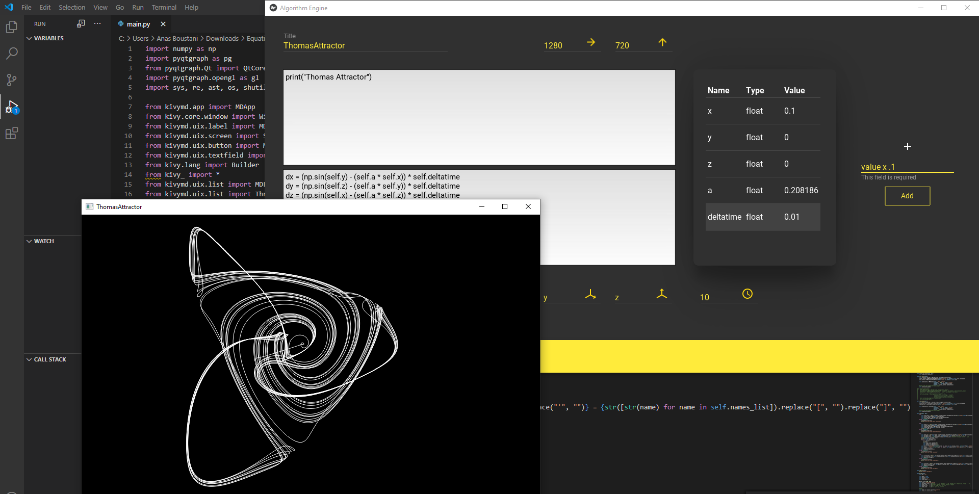
Let's begin with cloning this repository: git clone https://github.com/MrSinho/function-engine

open the terminal with the virtual environment activated, and type

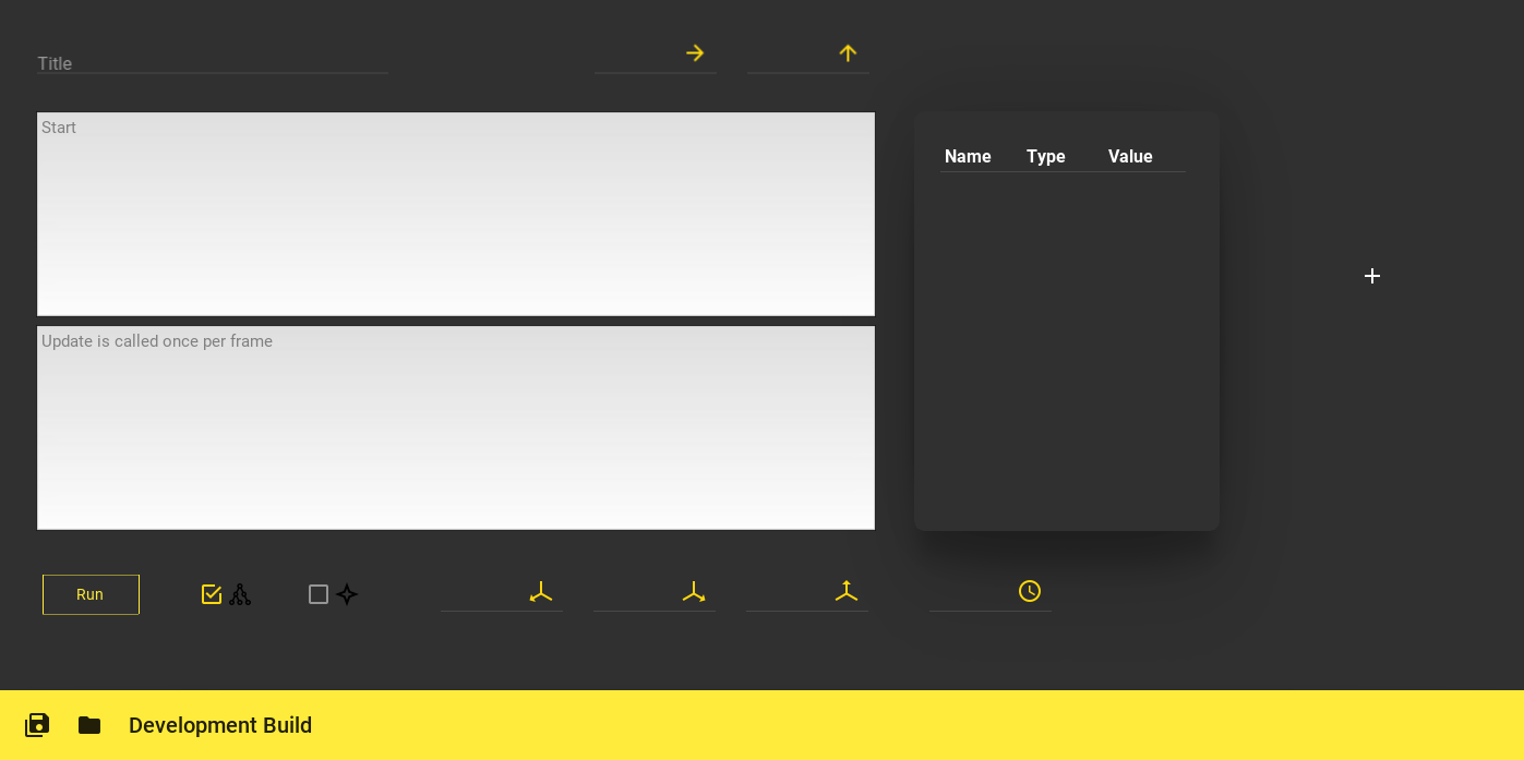
python -m pip install -r requirements.txt

Now run the main.py, you'll see something like this:

Overview

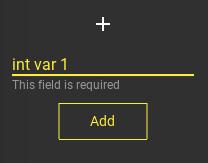
In the Start function you have to write some basic code which will run just at the beginning of the script, here you can also import custom libraries; the Update function runs/is updated every time your machine makes a new frame. On the left you have the variables data table, which contains the variables you're going to use. If you click the plus icon, you can add, rename, and change the type and value of a variable. Example:

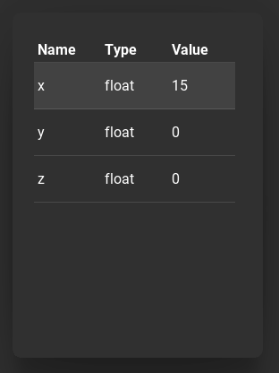
We want to add a variable var, so we have to give the type name and the initial value or var: int var = 1
Now let's rename it to x: rename var x
We also need to change the value to float: type x float
The initial value is too small, we want something bigger: value x 15

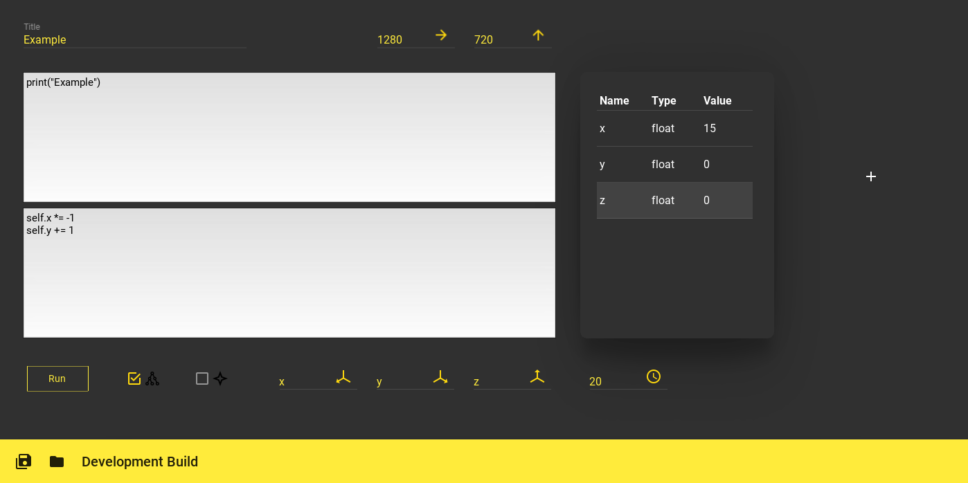
Let's write our first equation: first, we need to add more variables, click on the plus icon, and write float y = 1, float z = 0.

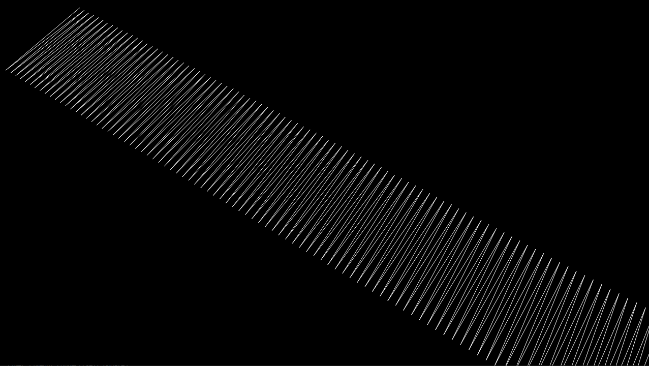
In the Start function we'll print the name of the equation, just for fun: print("Example"). In the Update function we'll turn x to negative, then to positive, and so on... self.x *= -1, and y will slowly increase by 1 self.y += 1 So this is the final result:

self.x *= -1
self.y += 1

We have to specify which variables will represent which axis: for now the x will represent the x axis, the y for the y axis and the z for the z axis.

You'll also notice an input field with a clock icon on the right: this represents the update delay in milliseconds, which means how fast will the code update. We'll give an input of 20 milliseconds.

We also have to choose what to see in the three-dimensional graph: some lines, or some dots? Let's select the first option for drawing lines. Note: the dots option is not fully optimized.

If you go up you'll see there are some more required field: the one on the upper left corner is the title of what we're doing, I'll type Example inside. On the right, the other ones tell the default width and height of the window with the 3d environment. Let's make a width of 1280 pixels and a height of 720 pixels.

Before running, let's save what we've done: click on the save icon of the toolbar (down left corner), then give a name to the code:

Now execute the code by clicking the Run button.

This is the final result:

Load some examples

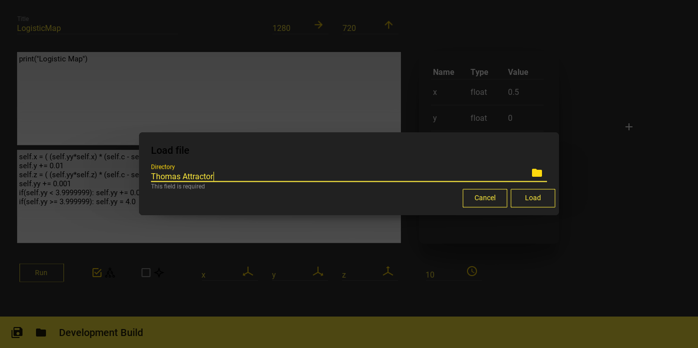
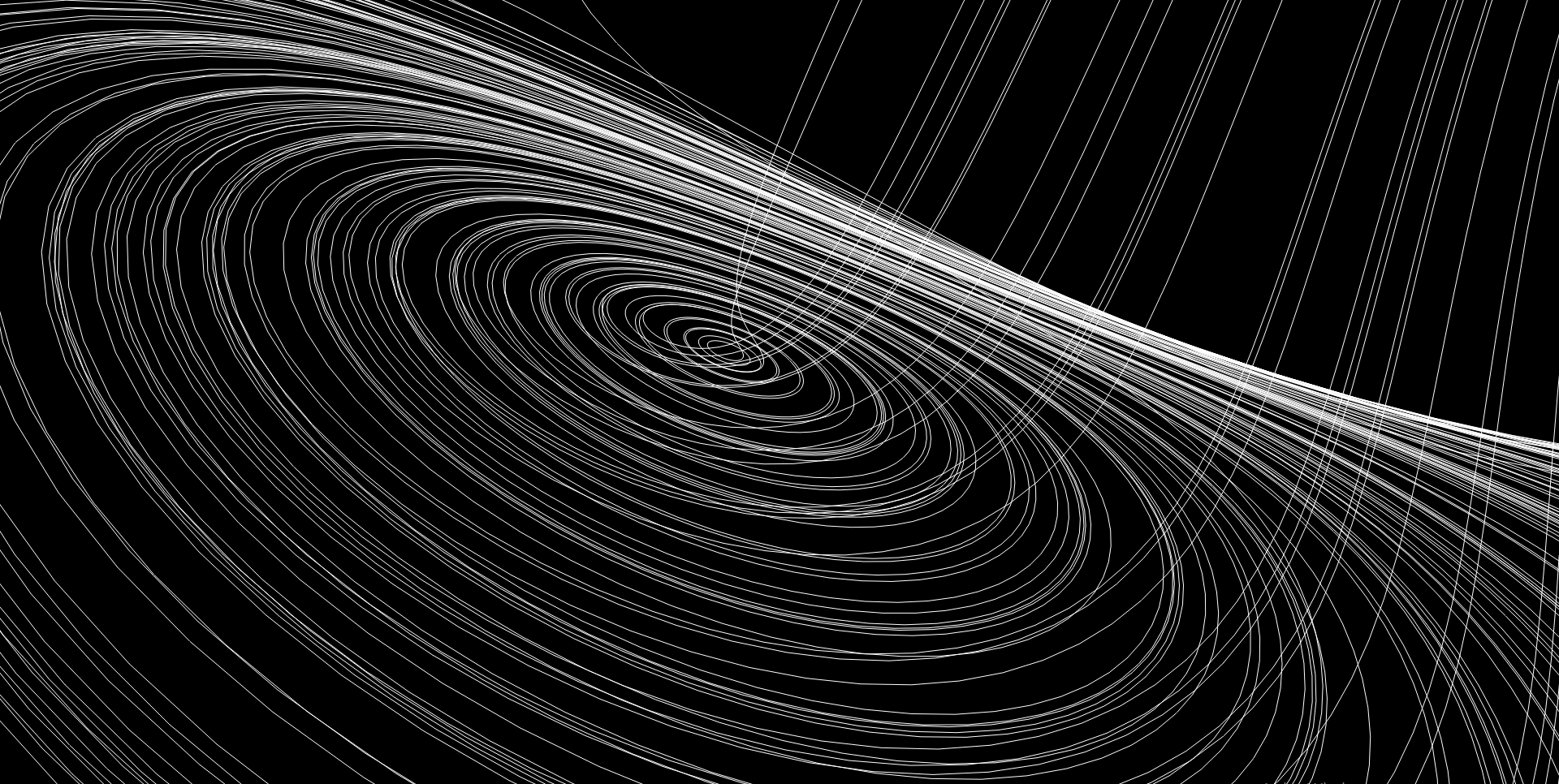
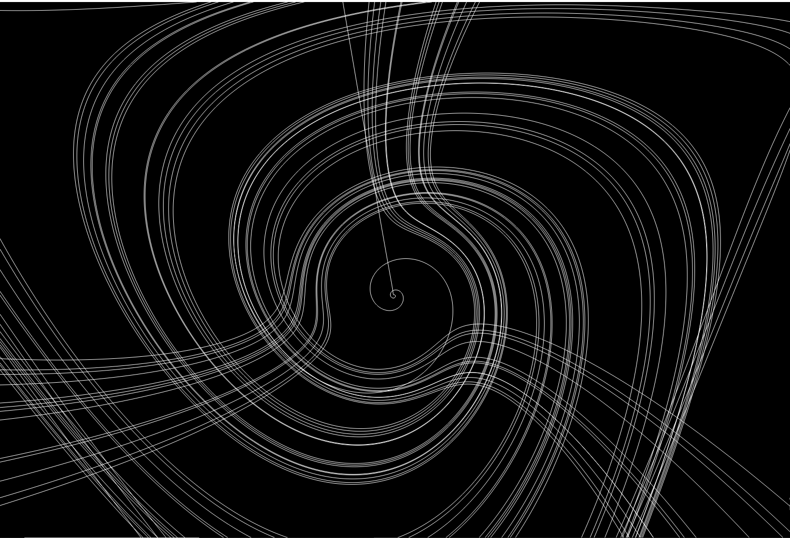
You can load (by clicking the folder icon on the toolbar) more examples, such as the Lorenz Attractor, the Thomas Attractor, and the Logistic Map, which are on this repository by default. You can also write, save, and load your equations.

Made by MrSinho