coronavirus

The coronavirus package provides a tidy format dataset of the 2019 Novel Coronavirus COVID-19 (2019-nCoV) epidemic. The raw data pulled from the Johns Hopkins University Center for Systems Science and Engineering (JHU CCSE) Coronavirus repository.

More details available here, and a csv format of the package dataset available here

Source: Centers for Disease Control and Prevention’s Public Health Image Library

Important Note

As this an ongoing situation, frequent changes in the data format may occur, please visit the package news to get updates about those changes

Installation

Install the CRAN version:

install.packages("coronavirus")

Install the Github version (refreshed on a daily bases):

# install.packages("devtools")
devtools::install_github("RamiKrispin/coronavirus")

Data refresh

While the coronavirus CRAN version is updated every month or two, the Github (Dev) version is updated on a daily bases. The update_dataset function enables to overcome this gap and keep the installed version with the most recent data available on the Github version:

library(coronavirus)
update_dataset()

Note: must restart the R session to have the updates available

Alternatively, you can pull the data using the Covid19R project data standard format with the refresh_coronavirus_jhu function:

covid19_df <- refresh_coronavirus_jhu()

head(covid19_df)
#>         date    location location_type location_code location_code_type     data_type value      lat      long
#> 1 2020-06-03 Afghanistan       country            AF         iso_3166_2     cases_new   758 33.93911 67.709953
#> 2 2020-06-07 Afghanistan       country            AF         iso_3166_2 recovered_new    45 33.93911 67.709953
#> 3 2020-06-02 Afghanistan       country            AF         iso_3166_2     cases_new   759 33.93911 67.709953
#> 4 2020-06-04 Afghanistan       country            AF         iso_3166_2     cases_new   787 33.93911 67.709953
#> 5 2020-06-08 Afghanistan       country            AF         iso_3166_2 recovered_new   296 33.93911 67.709953
#> 6 2020-06-06 Afghanistan       country            AF         iso_3166_2 recovered_new    68 33.93911 67.709953

Dashboard

A supporting dashboard is available here

Usage

data("coronavirus")

This coronavirus dataset has the following fields:

date - The date of the summary
province - The province or state, when applicable
country - The country or region name
lat - Latitude point
long - Longitude point
type - the type of case (i.e., confirmed, death)
cases - the number of daily cases (corresponding to the case type)

head(coronavirus)
#>         date province     country      lat      long      type cases
#> 1 2020-01-22          Afghanistan 33.93911 67.709953 confirmed     0
#> 2 2020-01-23          Afghanistan 33.93911 67.709953 confirmed     0
#> 3 2020-01-24          Afghanistan 33.93911 67.709953 confirmed     0
#> 4 2020-01-25          Afghanistan 33.93911 67.709953 confirmed     0
#> 5 2020-01-26          Afghanistan 33.93911 67.709953 confirmed     0
#> 6 2020-01-27          Afghanistan 33.93911 67.709953 confirmed     0

Summary of the total confrimed cases by country (top 20):

library(dplyr)

summary_df <- coronavirus %>% 
  filter(type == "confirmed") %>%
  group_by(country) %>%
  summarise(total_cases = sum(cases)) %>%
  arrange(-total_cases)

summary_df %>% head(20) 
#> # A tibble: 20 x 2
#>    country        total_cases
#>    <chr>                <int>
#>  1 US                 5141208
#>  2 Brazil             3057470
#>  3 India              2329638
#>  4 Russia              895691
#>  5 South Africa        566109
#>  6 Mexico              492522
#>  7 Peru                483133
#>  8 Colombia            410453
#>  9 Chile               376616
#> 10 Iran                331189
#> 11 Spain               326612
#> 12 United Kingdom      313394
#> 13 Saudi Arabia        291468
#> 14 Pakistan            285191
#> 15 Bangladesh          263503
#> 16 Argentina           260911
#> 17 Italy               251237
#> 18 Turkey              243180
#> 19 France              239355
#> 20 Germany             219540

Summary of new cases during the past 24 hours by country and type (as of 2020-08-11):

library(tidyr)

coronavirus %>% 
  filter(date == max(date)) %>%
  select(country, type, cases) %>%
  group_by(country, type) %>%
  summarise(total_cases = sum(cases)) %>%
  pivot_wider(names_from = type,
              values_from = total_cases) %>%
  arrange(-confirmed)
#> # A tibble: 188 x 4
#> # Groups:   country [188]
#>    country            confirmed death recovered
#>    <chr>                  <int> <int>     <int>
#>  1 India                  60963   834     56110
#>  2 US                     46808  1074     44205
#>  3 Colombia               12830   321      8943
#>  4 Argentina               7043   240     73147
#>  5 Mexico                  6686   926      4118
#>  6 Russia                  4892   130      6479
#>  7 Spain                   3632     5         0
#>  8 Iraq                    3396    67      2312
#>  9 Bangladesh              2996    33      1535
#> 10 Philippines             2900    18       273
#> 11 South Africa            2511   130      8925
#> 12 Iran                    2345   184      1978
#> 13 Israel                  1871     9      1082
#> 14 Bolivia                 1693    49       930
#> 15 Indonesia               1693    59      1474
#> 16 Chile                   1572    39      2199
#> 17 Saudi Arabia            1521    34      1640
#> 18 Romania                 1215    35       274
#> 19 Ukraine                 1211    29       590
#> 20 Turkey                  1183    15      1185
#> 21 Venezuela               1138     9      2776
#> 22 Morocco                 1132    17       861
#> 23 Panama                  1070    16      1155
#> 24 Germany                 1032     5       965
#> 25 Guatemala                979    11       853
#> 26 Ecuador                  862    19         2
#> 27 Kazakhstan               691   211       975
#> 28 Japan                    685     6       686
#> 29 Kuwait                   668     4       731
#> 30 Nepal                    638     4       171
#> 31 Costa Rica               636    11       148
#> 32 Dominican Republic       595    18       756
#> 33 Ethiopia                 584    20       285
#> 34 Poland                   551    12       273
#> 35 Honduras                 531     9       156
#> 36 Pakistan                 531    15       482
#> 37 Kenya                    497    15       372
#> 38 Algeria                  492    10       343
#> 39 Uzbekistan               443     4       712
#> 40 Nigeria                  423     6       263
#> # … with 148 more rows

Plotting the total cases by type worldwide:

library(plotly)

coronavirus %>% 
  group_by(type, date) %>%
  summarise(total_cases = sum(cases)) %>%
  pivot_wider(names_from = type, values_from = total_cases) %>%
  arrange(date) %>%
  mutate(active = confirmed - death - recovered) %>%
  mutate(active_total = cumsum(active),
                recovered_total = cumsum(recovered),
                death_total = cumsum(death)) %>%
  plot_ly(x = ~ date,
                  y = ~ active_total,
                  name = 'Active', 
                  fillcolor = '#1f77b4',
                  type = 'scatter',
                  mode = 'none', 
                  stackgroup = 'one') %>%
  add_trace(y = ~ death_total, 
             name = "Death",
             fillcolor = '#E41317') %>%
  add_trace(y = ~recovered_total, 
            name = 'Recovered', 
            fillcolor = 'forestgreen') %>%
  layout(title = "Distribution of Covid19 Cases Worldwide",
         legend = list(x = 0.1, y = 0.9),
         yaxis = list(title = "Number of Cases"),
         xaxis = list(title = "Source: Johns Hopkins University Center for Systems Science and Engineering"))

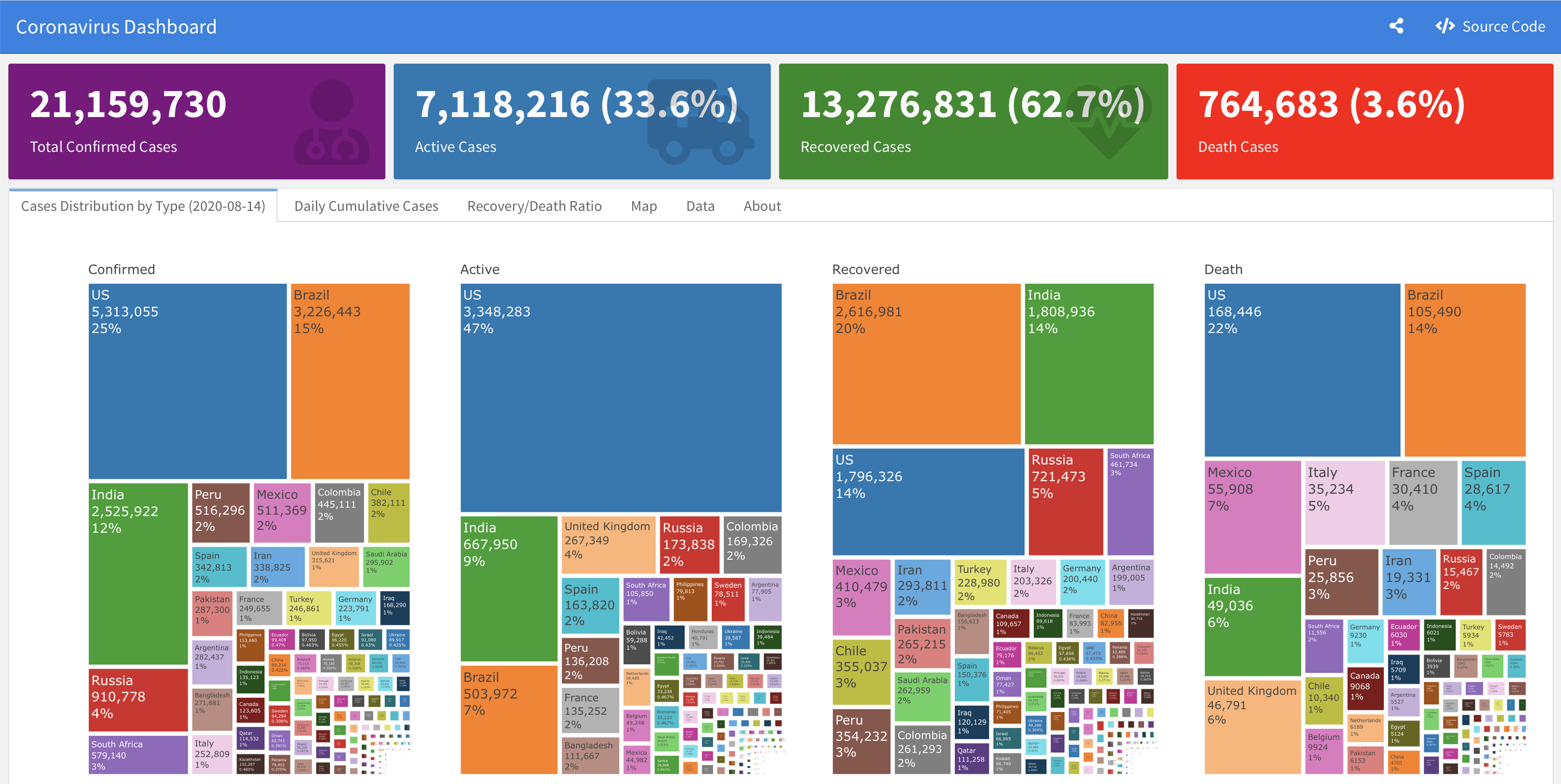
Plot the confirmed cases distribution by counrty with treemap plot:

conf_df <- coronavirus %>% 
  filter(type == "confirmed") %>%
  group_by(country) %>%
  summarise(total_cases = sum(cases)) %>%
  arrange(-total_cases) %>%
  mutate(parents = "Confirmed") %>%
  ungroup() 
  
  plot_ly(data = conf_df,
          type= "treemap",
          values = ~total_cases,
          labels= ~ country,
          parents=  ~parents,
          domain = list(column=0),
          name = "Confirmed",
          textinfo="label+value+percent parent")

Data Sources

The raw data pulled and arranged by the Johns Hopkins University Center for Systems Science and Engineering (JHU CCSE) from the following resources:

World Health Organization (WHO): https://www.who.int/
DXY.cn. Pneumonia. 2020. http://3g.dxy.cn/newh5/view/pneumonia.
BNO News: https://bnonews.com/index.php/2020/02/the-latest-coronavirus-cases/
National Health Commission of the People’s Republic of China (NHC):
http:://www.nhc.gov.cn/xcs/yqtb/list_gzbd.shtml
China CDC (CCDC): http:://weekly.chinacdc.cn/news/TrackingtheEpidemic.htm
Hong Kong Department of Health: https://www.chp.gov.hk/en/features/102465.html
Macau Government: https://www.ssm.gov.mo/portal/
Taiwan CDC: https://sites.google.com/cdc.gov.tw/2019ncov/taiwan?authuser=0
US CDC: https://www.cdc.gov/coronavirus/2019-ncov/index.html
Government of Canada: https://www.canada.ca/en/public-health/services/diseases/coronavirus.html
Australia Government Department of Health: https://www.health.gov.au/news/coronavirus-update-at-a-glance
European Centre for Disease Prevention and Control (ECDC): https://www.ecdc.europa.eu/en/geographical-distribution-2019-ncov-cases
Ministry of Health Singapore (MOH): https://www.moh.gov.sg/covid-19
Italy Ministry of Health: http://www.salute.gov.it/nuovocoronavirus
1Point3Arces: https://coronavirus.1point3acres.com/en
WorldoMeters: https://www.worldometers.info/coronavirus/
COVID Tracking Project: https://covidtracking.com/data. (US Testing and Hospitalization Data. We use the maximum reported value from “Currently” and “Cumulative” Hospitalized for our hospitalization number reported for each state.)
French Government: https://dashboard.covid19.data.gouv.fr/
COVID Live (Australia): https://www.covidlive.com.au/
Washington State Department of Health: https://www.doh.wa.gov/emergencies/coronavirus
Maryland Department of Health: https://coronavirus.maryland.gov/
New York State Department of Health: https://health.data.ny.gov/Health/New-York-State-Statewide-COVID-19-Testing/xdss-u53e/data
NYC Department of Health and Mental Hygiene: https://www1.nyc.gov/site/doh/covid/covid-19-data.page and https://github.com/nychealth/coronavirus-data
Florida Department of Health Dashboard: https://services1.arcgis.com/CY1LXxl9zlJeBuRZ/arcgis/rest/services/Florida_COVID19_Cases/FeatureServer/0 and https://fdoh.maps.arcgis.com/apps/opsdashboard/index.html#/8d0de33f260d444c852a615dc7837c86
Palestine (West Bank and Gaza): https://corona.ps/details
Israel: https://govextra.gov.il/ministry-of-health/corona/corona-virus/
Colorado: https://covid19.colorado.gov/covid-19-data