title: Random Forests in Python author: name: Nathan Epstein twitter: epstein_n url: http://nepste.in email: _@nepste.in

Random Forests in Python

Model Internals
Examples
Forests vs. Neural Nets
AI Example

Model Internals

Ensemble machine learning model.
Composite of many simpler models called decision trees.
The individual trees are formed by branching on each of the included features. The random forest is an aggregation of these trees.

Decision Trees

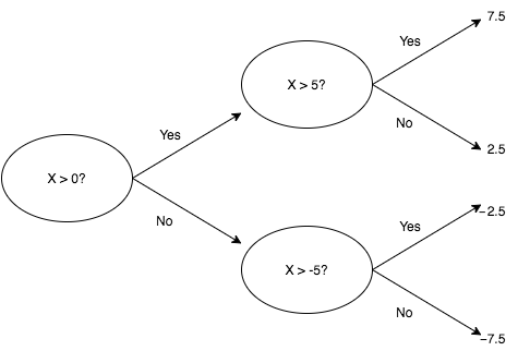
Decision trees branch on each of the included features in order to partition the data.
For each bin in the partition (i.e., leaf of the tree), we assign an output value to inputs contained in that bin.

Classification Trees

In a classification problem, the output is categorical.
Each branch of the tree (collection of feature values) leads to a different leaf (output value).

Example: Prisoner's Dilemma

Regression Trees

The leaves of the tree still form a partition of the output space, but there are many possible values within each bin.
How do we assign a single value? We take the mean among values assigned to that bin.

Example: |x| for x in (-10, 10)

Tree Order

It’s clear that the order of branches in a decision tree matters.
Less transparent is how the path to each leaf is constructed.
This happens according to an iterative approach called entropy minimization (greedy algorithm, branch on highest information gain feature at each step).

Tree Order

Unless you're familiar with information theory, the intuition behind entropy minimization may not be obvious.
Our problem is the following: given a set of features, how do we partition the output space as finely as possible, as quickly as possible? --

"Guess Who?"

An intuitive way to understand this challenge is the game “Guess Who?”.

"Guess Who?"

In "Guess Who?" players try to identify the opposing player's character from a pre-set list.
Individuals take turns asking yes or no questions to expose features about the character.

Low Information Gain

It’s typical to ask questions like whether the character “wears glasses” or “has white hair.”
These questions represent features with low information gain.
More likely than not, the answer will be no and we will have eliminated only a few possibilities.

High Information Gain

A higher information gain feature will partition the data as evenly as possible.
What if we just list half of the available characters and ask if the opponent's character is in that set (i.e., "is your character Bob, or Ted, or Jen, or ... ?").

High Information Gain

Membership in one-half of the characters is a feature which perfectly bisects the data
We are guaranteed to eliminate exactly half of the possibilities.
In the general case (of n characters), we can identify the target character with only log_2(n) operations.

Making a Forest from Trees

Forests from Trees

Overfitting is a well-known pitfall for decision trees.
For example, if we add an additional 1000 characters onto the board, asking about the 12 characters from before is a bad question and will almost certainly underperform “white hair.”

Forests from Trees

Overcoming this pitfall is the purpose of random forests.
To avoid overfitting with a single tree, we build an ensemble model through a procedure called bagging.

Ensemble Models

An ensemble model is a one made by combining other models.
The average of many unbiased predictors with high variance is an unbiased predictor with low(er) variance.

Bagging Procedure

For some number of trees, T, and predetermined depth, D, select a random subset of the data (convention is roughly 2/3 with replacement).
Train a decision tree on that data using a subset of the available features (roughly sqrt(M) by convention, where M is the total number of features).

Parameter Tuning

Obviously, these parameters can be tuned to fit the needs of the application.
A model with more trees / data can take longer to train, but may have greater accuracy.
More depth / features increases the likelihood of overfitting, but may be appropriate if features have complex interactions.

Classification / Regression Forests

In the case of a classification problem, we use the mode of the trees’ output to classify each value.
For regression problems, we use the mean of the output trees.
Note that the aggregation process is independent of the internal workings of the individual decision trees. Because each tree can make a prediction using the available features (or a subset thereof), they can be polled to form an aggregate prediction.

Avoiding Overfitting

It’s difficult to overfit with only a subset of the available information.
By building the random forest model as an aggregation of weaker models (weak in that the trees are trained on a subset of the available information), we are able to build a strongly predictive model while avoiding the pitfalls of overfitting.

Strong Suits

What makes random forests such an effective tool is their robustness to different types of data (e.g., non-linear / non-monotonic functions, un-scaled data, data with missing values, data with poorly chosen features).
This makes them an excellent “out of the box” tool for general machine learning problems which do not immediately suggest themselves to a specific alternative.

Examples

Non-linear Functions

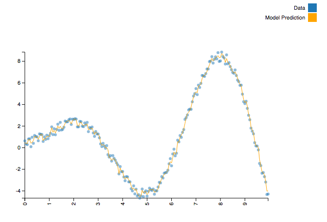
Consider a function like y = x⋅sin(x) + U, where U is a random value uniformly distributed in the interval (0, 1).
It’s a “simple” function, but it is both non-monotonic and non-linear.
A technique like simple regression is a non-starter without significant feature extraction. However, it is a simple task for a random forest.

Non-linear Functions

from sklearn.ensemble import RandomForestRegressor
import numpy as np
import math

def generate_data():
        X, Y = [], []
        f = lambda x : x * math.sin(x) + np.random.uniform()
        for x in np.arange(0, 10, 0.05):
                X.append([x])
                Y.append(f(x))
        return (X, Y)

X, Y = generate_data()
model = RandomForestRegressor()
model = model.fit(X, Y)

Unscaled Features

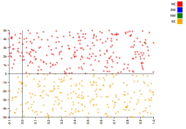
Consider the following example. We will seek to classify points as being within four quadrants: “NE” (x > 0 and y > 0), “NW” (x < 0 and y > 0), “SE” (x > 0 and y < 0), and “SW” (x < 0 and y < 0).
A straightforward example, except that our x values will cover the interval (-0.1, 1), while our y values will cover the interval (-5000, 5000).

Unscaled Features

import numpy as np
from sklearn.ensemble import RandomForestClassifier
import math

def quadrant(coords):
        EW = 'W' if coords[0] < 0 else 'E'
        NS = 'S' if coords[1] < 0 else 'N'
        return NS + EW

N = 10000
x = -0.1 + np.random.sample(N) * 1.1
y = -5000 + np.random.sample(N) * 10000

xy_coords = list(zip(x, y))
quadrant = list(map(quadrant, xy_coords))

model = RandomForestClassifier()
model = model.fit(xy_coords, quadrant)

K-Nearest Neighbors...

Forests vs. Neural Nets

Neural Nets

In a time when neural networks are as popular as they are, it’s tempting to ask why any of this matters. Why not just use neural nets?

Why not Neural Nets?

Parameter tuning tends to be simpler with forests; there are well established conventions for choosing parameters in random forests, but how to determine network layer structure is fairly opaque.

Why not Neural Nets?

There is a more robust body of academic literature around them which makes the internal workings (arguably) easier to understand.

Why not Neural Nets?

Generally simpler to implement. Popular implementations (e.g., scikit-learn) allow users to train sensible random forests with as little as a single line of code. Configuring network layer architecture generally involves more set up.

Why not Neural Nets?

Random forests are inherently parallelizable and extremely well supported for distributed deployment. Through MLlib, random forests are included in Apache Spark and are therefore easily scalable.

AI with Random Forests

AI Search

Given an array of sorted numbers, we would like to find a target value as quickly as possible.
Our random numbers will be distributed exponentially. Can we use this information to do better than binary search?

Approach

Create many example searches (random, linear, and binary).
For each step in the searches, create an observation.
Input will be a tuple of current index, known floor, known ceiling, current value / target value (i.e. { 'location': 10, 'floor': 5, 'ceil': 12, 'ratio': 1.5 }).
Output will be the desired step size to locate the target value.

Training

simulator = SearchSimulation()
training_data = simulator.observations(TRAINING_SIZE, ARRAY_SIZE)

states = pd.DataFrame(training_data['states'])
deltas = pd.DataFrame(training_data['deltas'])

model = RandomForestClassifier()
model = model.fit(states, deltas)

class AISearch(Search):
  def update_location(self):
    self.location += model.predict(self.state())[0]

Code can be found at https://github.com/NathanEpstein/pydata-london

Results

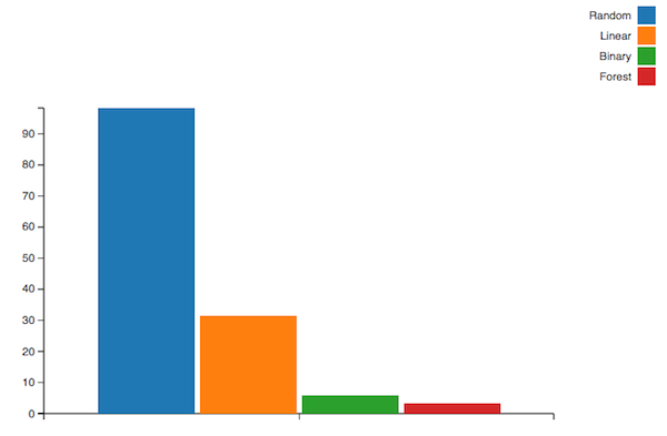
random: 98.34, linear: 31.5, binary: 5.87, AI: 3.32

Binary vs. Forest