This project aims to reobtain the results presented in Machine learning phases of matter (Juan Carrasquilla, Roger G. Melko) regarding the two-dimensional square Ising model. The authors show that a standard feed-forward neural network (FFNN) is a suitable tool to detect Ising's model phase transition.
This is done by first comparing the behavior of a fully connected neural networr (FCNN) to a hand-made Toy model.
Then the number of parameters of the FCNN is increased and the accuracy of the model is studied as a function of the lattice size to remove boundary effects. In the original article, the FCNN is then upgraded to a convolutional neural network to test its accuracy on non-Ising Hamiltonians.
Finally, as an appendix, the original data is analyzed with the t-stochastic neighbors embedding algorithm to separate the data into clusters.
❕ The project is subdivided into notebook written to be run on google colab. A copy is provided in this repository but they may not run in your local environment. It is possible to access the original notebooks using the link provided.
The following sections present a summary of the results obtained. A detailed discussion is available inside the notebooks themselves.
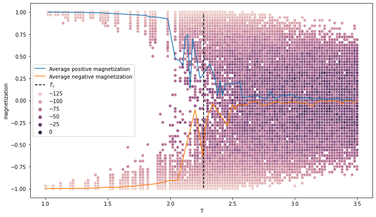
The first notebook is centered around the Monte Carlo code MonteCarloSampling.c written to generate the configurations.
In particular, in the notebook the behavior of the magnetization and the autocorrelation will be analyzed. Both tests will lead to positive results with a correlation length of
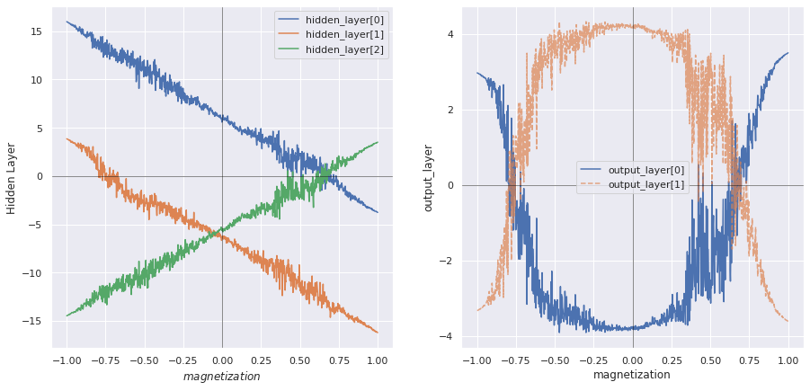
The second notebook focuses on the Toy Model presented in the article and examines the corresponding FCNN. The analytical toy model correctly classifies the temperature up to a parameter
- Input layer consisting of
$L^2$ neurons; - Hidden layer with 3 neurons and a sigmoid activation function;
- Output layer with 2 neurons and a sigmoid activation function.
The activation function was switched from Heaviside to Sigmoid as suggested in the article to avoid the pathological behavior of the Heaviside's gradient.
The network's performances have a high dependence on the stochastic component of the training. If the training goes well the test loss is smaller than 0.1 percent, otherwise, it oscillates between 0.2 and 0.4 (this problem will be solved in the third notebook). When the training goes well both the hidden layer and the output layer provide similar results to the toy model and the critical temperature is correctly identified within a small error.
The third notebook will be more theory-oriented. First, the Toy model FCNN will be upgraded with a hidden layer of 100 neurons, then the training procedure will be discussed in detail. Following that, the results of Juan Carrasquilla and Roger G. Melko on non-standard Ising hamiltonian will be presented.
The fourth notebook will try to implement the content of Appendix B: Visualizing the action of a neural network on the Ising ferromagnet using scikit-learn's implementation of t-SNE.
Results for various values of perplexity
As t-SNE uses a non-convex cost function the plot will always look different. Some plots obtained are reported for clarity. As they were obtained by repetitive runs until a "good-looking" plot was produced, they have little scientific meaning.
- Perplexity 100; Early Exaggeration 195
- Perplexity 100; Early Exaggeration 50; points around
$T_C$ used
- Perplexity 50; Early Exaggeration 50; points around
$T_C$ used
- Perplexity 30; Early Exaggeration 50; points around
$T_C$ used
- Perplexity 10; Early Exaggeration 50; points around
$T_C$ used
- Perplexity 4; Early Exaggeration 50; points around
$T_C$ used
- Article: Machine learning phases of matter, arxiv version available in the repository.
- Pytorch tutorials: https://pytorch.org/tutorials/
- Understanding binary cross-entropy / log loss: a visual explanation
- Differentiable Programming from Scratch: article on the inner working mechanism of the automatic differentiation algorithm of PyTorch.
- Adam: A Method for Stochastic Optimization: arXiv entry for the Adam optimizer. Only the first two sections were consulted.
- Why Momentum really Works
- t-distributed stochastic neighbour embedding: Wikipedia entry for t-SNE
- How to Use t-SNE Effectively


