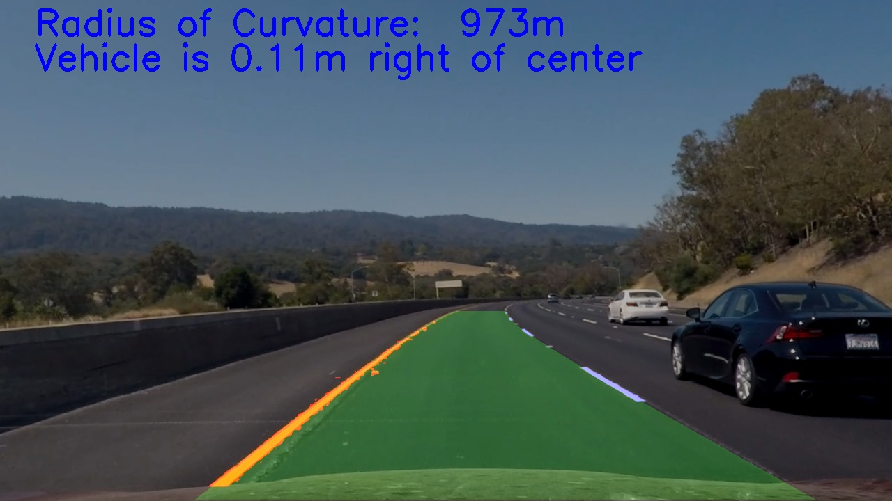
The steps of this project are the following:
- Compute the camera calibration matrix and distortion coefficients given a set of chessboard images.
- Apply a distortion correction to raw images.
- Use color transforms, gradients, etc., to create a thresholded binary image.
- Apply a perspective transform to rectify binary image ("birds-eye view").
- Detect lane pixels and fit to find the lane boundary.
- Determine the curvature of the lane and vehicle position with respect to center.
- Warp the detected lane boundaries back onto the original image.
- Output visual display of the lane boundaries and numerical estimation of lane curvature and vehicle position.
All functions used for the processing are located in the file called Advanced_lane_detection.py in this repository.
The code for this step is contained in the functions compute_camera_calibration() and undistort_image() in lines 151 through 192.
First I prepare "object points", which will be the (x, y, z) coordinates of the chessboard corners in the world. Here I am assuming the chessboard is fixed on the (x, y) plane at z=0, such that the object points are the same for each calibration image. Thus, objp is just a replicated array of coordinates, and objpoints will be appended with a copy of it every time I successfully detect all chessboard corners in a test image. imgpoints will be appended with the (x, y) pixel position of each of the corners in the image plane with each successful chessboard detection.
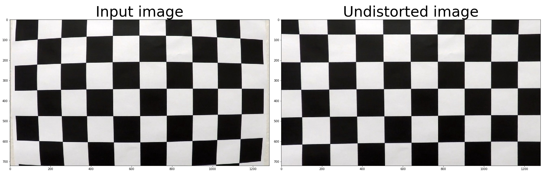
I then use the output objpoints and imgpoints to compute the camera calibration and distortion coefficients using the cv2.calibrateCamera() function. I applied this distortion correction to the test image using the cv2.undistort() function and obtained this result:
In this step I use the distortion coefficients from the calibration step and undistort_image() to undistort the input image. This is the result of the undistortion for one of the input images:
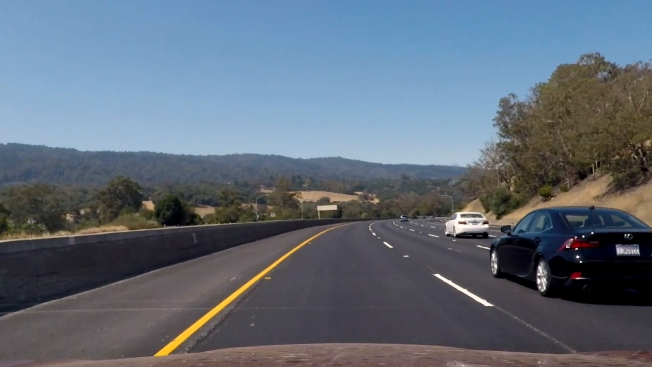
For seperating the lane markings from the background I convert the input image into the HSL color space and use a combination of thresholds on different color channels to generate a binary image (thresholding steps in function image_to_thresholded_binary() at lines 269 through 287 and extract_single_color() at lines 195 through 210). This way I can detect the white lane markings by thresholding based on the L (lightness) value. To improve detection of the yellow lane markings filtering the image by the corresponding H (hue) values helps for a good detection especially in darker areas (shadows etc.). The result of both thresholded images are then combined. Here's an example of the output for this step:
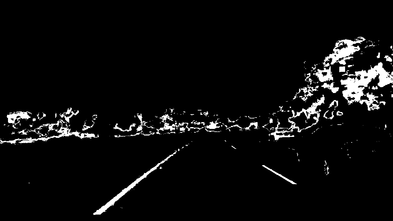 As you can see the lane markings are selected and the rest of the street got cut out quite nicely, particularly in the region of interest which is our lane. There are other detections that are outside of our ROI, such as the landscape in the background and detections of the cars on other lanes. We do not have to worry about these detections because these parts of the image will get cut out in the perspective transform which is the next step in the pipeline.
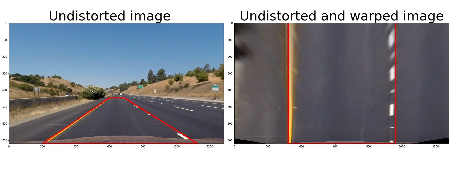
The code for my perspective transform includes a function called warp() (which appears in lines 290 through 301). This warp() function takes as inputs an image (img), as well as source (src) and destination (dst) points. I choose to select and hardcode the source and destination points in the following manner to cut out the relevant ROI:
src = np.float32(
    [165, img.shape[0]],
    [596,447],
    [681,447],
    [1124,img.shape[0]],
dst = np.float32(
    [300,img.shape[0]],
    [300,0],
    [950,0],
    [950,img.shape[0]],
This results in the following source and destination points:
| Source | Destination |
|---|---|
| 165, 720 | 300, 720 |
| 596, 447 | 300, 0 |
| 681, 447 | 950, 0 |
| 1124, 720 | 950, 720 |
I verify that my perspective transform is working as expected by drawing the src and dst points onto a test image and its warped counterpart to verify that the lines appear parallel in the warped image.
Now I have detected the lane markings and warped the input image to "birds-eye view". As next step I want to identify the pixels that are part of the left and right lane-markings to fit a polynomial. For this we can use two different approaches dependent on if we have a prior detection or not.
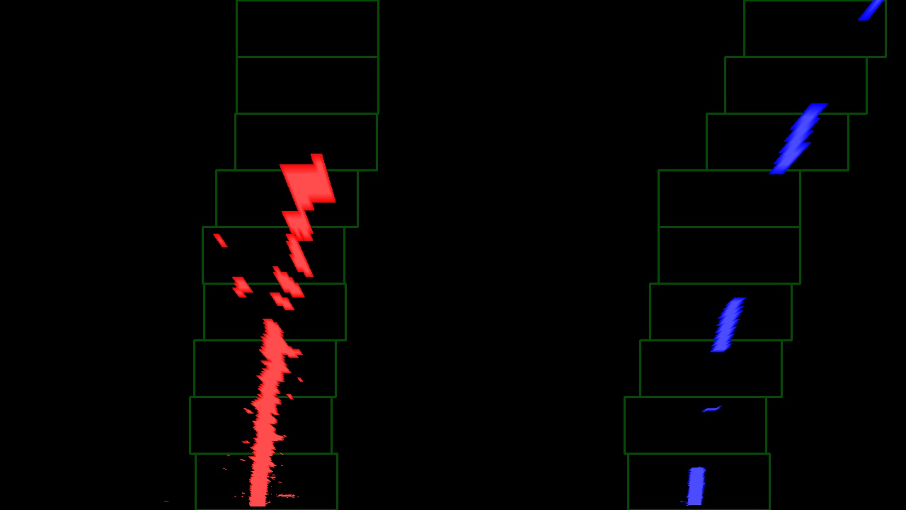
For seperating the left and right lane-markings I devide the image vertically (along the y-axis) in the middle of the image. Then I calculate the horizontal histogramms at the bottom of the picture to extract the peak for the left and the right half. The peaks correspond to our left and right markings respectively are now the starting point of the search for the lane-markings along the y-axis. For finding all pixels that can be part of the lane-markings now step by step I select all pixels above that are in a margin (box) centered from my last detection. After that I have all relevant pixel for left and right and I can fit a second order polynom with numpy's polyfit() function each. In my code this is triggered in the functions detect_lines() and this search is done by function search_new_polynomial_from_scratch() from line 365 to line 395. Here is an example image with the selected pixels, the search boxes and the fittet polylines:
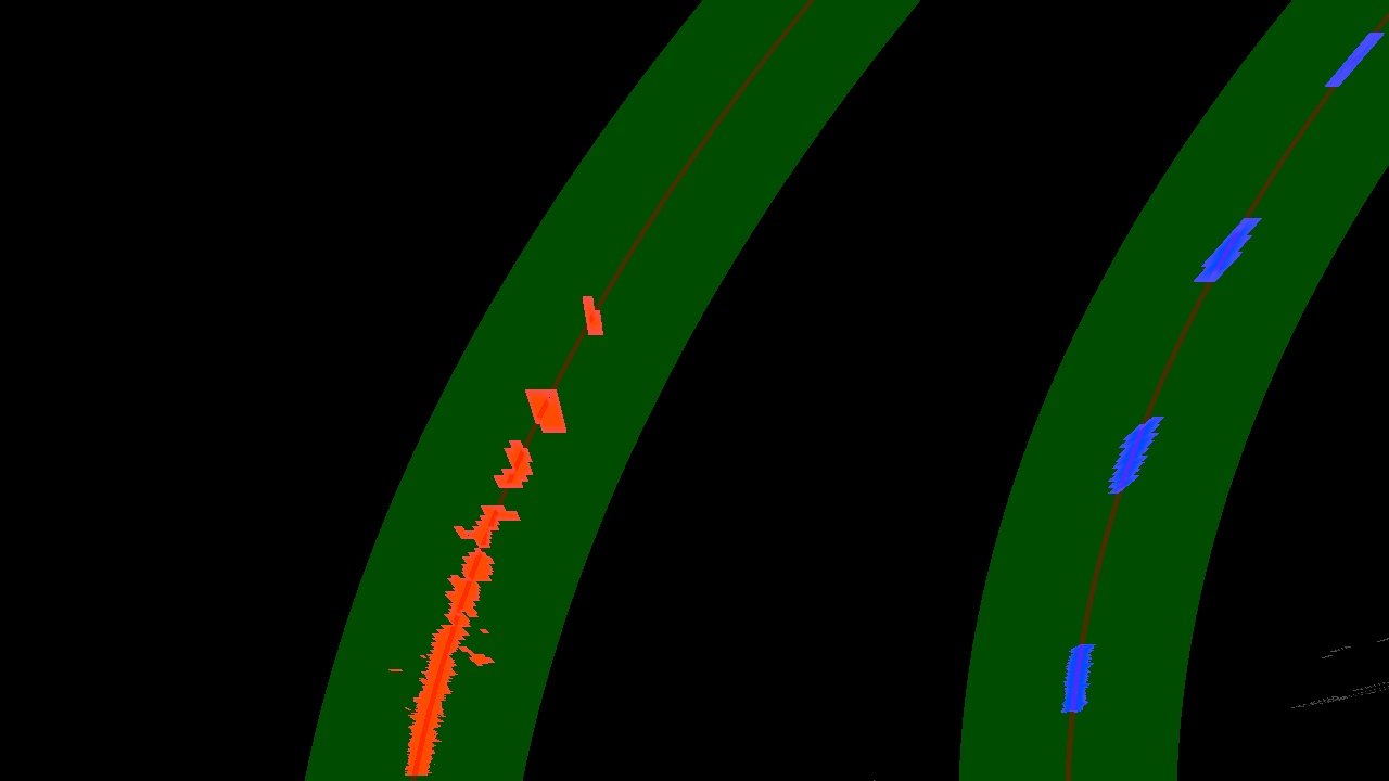
In the case that we have already found polylines before, we do not have to search from scratch again. We can search along the prior detected polylines and save processing time. For this I add a margin aroung the prior polylines and select all pixels within - highlighted by the green area. Then I can fit my new polylines again - which are visualized as brown lines. In my code this is done in the search_polynomial_from_prior() function. The approach to search from a prior polynom can result in a bad detection so I implemented a check if the new polylines make sence (in the code from line 548 to 575, which gets triggered by the function validation_check_line() ). This check compares the fitted line against the last 10 detections (realised with a line class in line 35 to 132 that stores the last 10 fitted lines). The output of the search from prior is displayed in the following image:
After fitting the left and the right polyline I do an additional sanity check if the left and right line actually represent a lane line. The function validation_check_lane() (line 572-575) triggers this check and compares the curvature as well as the distance of both polylines. If the lines are not valid I do another check for each the left and right line against the prior lines. To check if a line is not valid I use the average over the last 10 successfully fitted lines.
I calculate the lane curvature based on the polynom coefficients of the lines. The curvature of the polylines from one image to the next has a big jitter. To display a more reliable curvature of the lane I store the last 30 curvature values in the line class and calculate the average to get a smooth curvature value. I chose such a high value because the curvature of lanes change slowly and to reduce the jitter in the output to make the value better readable. The calculation of the curvature is done within the line class each time it gets updated with new value (line 101 to 114 in the code).
For calculating the position of the vehicle I calculate the middle point of the lane in front of the car. Based on the assumption that the camera is mounted centered on the car I calculate the offset between the middle of the road and where the middle of the picture is (taking the transformation into account). This is done in the calc_offset_lane_markings_center() function from line 691 to line 698.
For displaying the result of the lane detection I warped the detected markings and lane back onto the road. Function warp_back_on_original() (line 642 through 662) processes the warp and overlays the detection on the undistorted input image with opencv's addWeighted() function. In function warp_back_on_original() the calculated curvature and offset is annotated on the result image. Here is the result of my lane detection:
Here's a link to my video result
For the seperation of the lane markings from the rest of the image I tried different approaches. I tried gradient and canny-edge detection with different threshold based on grayscale images and also different color channels. With different threshold values I could not acchieve a good and stable detection of the lane markings without much detections in the environment. This was particularly bad in special lightning and road conditions.
In the end, I got the best result with the chosen combination of color channels and threshold. The biggest disadvantage here is that in some frames I do not get valid detection of enough lane-marking pixels. In some light conditions the yellow markings and their background get selected both as lane and bad polylines are the result. To solve this issue I implemented the validity check of the lane and the polylines so in these frames the detection can fall back to the average of the last fitted lines. But the thresholds depend really much on the whole environment conditions and did not perform good in the challenge videos.
Another disadvantage that remains is that I have to choose thresholds that reliably detect the yellow line which also lead to many small, noisy detections around to the lines which can impact the line fitting.
As mentioned before, this implementation relies heavily on smoothing to get a relilable lane detection. This comes with the disadvantage that the result of the detection lags a few frames behind. This is especially observable when the car drives over bumps in the road and in tighter curves. This might be a problem depending on the road-szenarios the car is driving and the detection accuracy requirements.
The developed architecture updates the lines only after the lane validity check. Therefore, there are quite some checker functions and fall back functions involved which leads to quite some possible control flow paths. This makes it more difficult to follow the code and to debug problems.
