Case Studies

Airbnb - EDA
Buildzoom - Classification
DataRobot - Classification

1. Airbnb

1.1 Problem

The product and operations team at Airbnb wants a detailed analysis of their guest host matching system in an attempt to grow bookings at Rio. The team wants to

Track a few KPI's that would help them monitor the success of the teams efforts in improving guest host matching.
Gain a deeper understanding of what areas to invest. Come up with a few recommendations, business initiative and product changes and demonstrate the rationale behind the recommendations.

1.2 Analysis

1.2.1 KPI's

Conversion rate (%)
- Across different stages of communication between guest & host, from first interation -> first reply -> acceptance -> booking/abandoned
- Across contact channel types (contact_me, book_it, instant_book)
- Across user type (New vs. Returning)
- Across room types (Private room vs. Entire Apt vs. Shared room)
Average time between interactions
- Across user-type and channel-type
# Interactions and # Characters in guests opening remark (Bookings vs. Abandoned)

1.2.2 Recommendations

Make suggestions to keep the interactions engaging

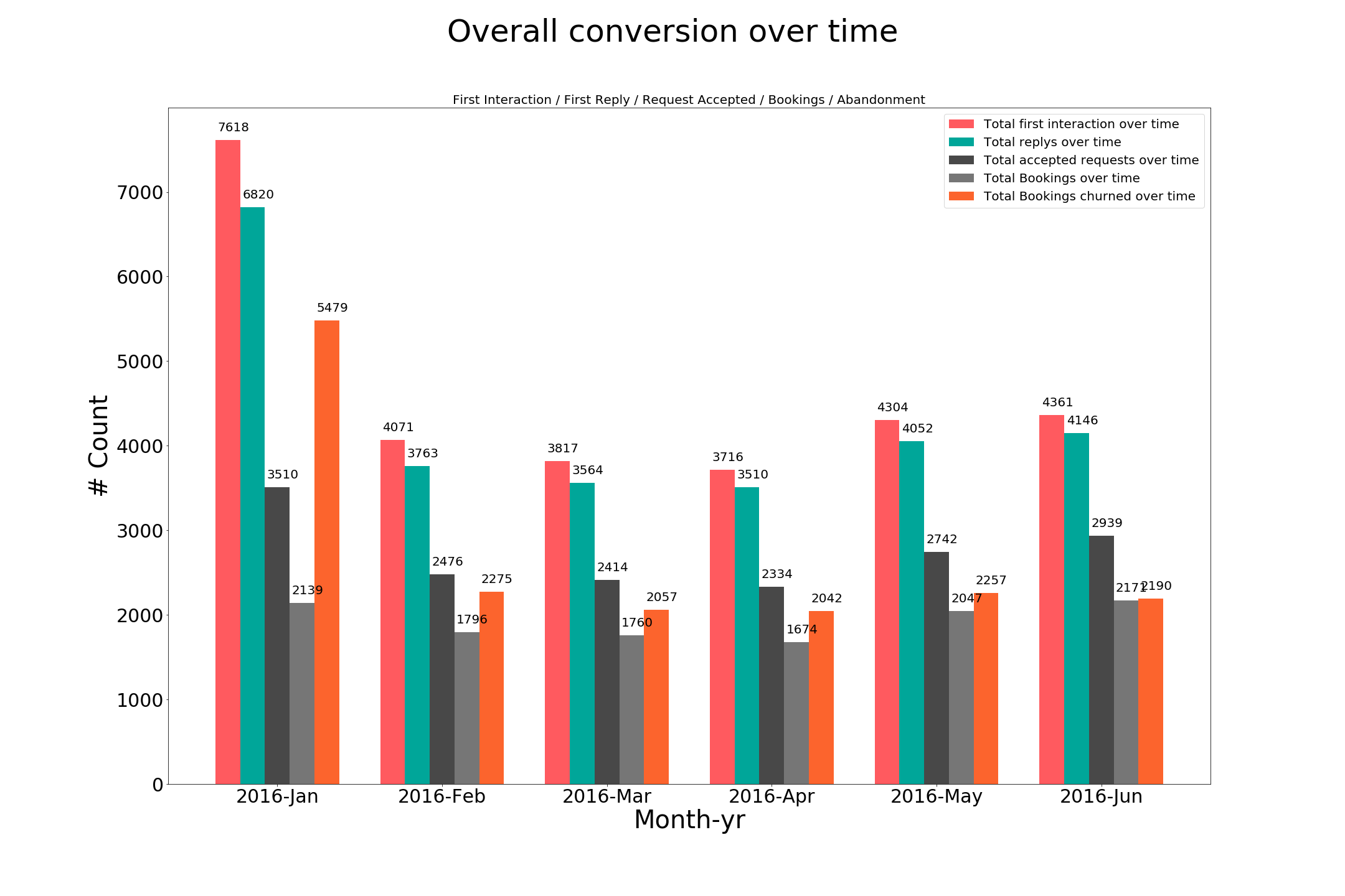
On an overall level, there is a massive drop in the number of accepted requests once we get past the reply phase. Providing sample suggestions to both guest and host could improve the chances of booking.

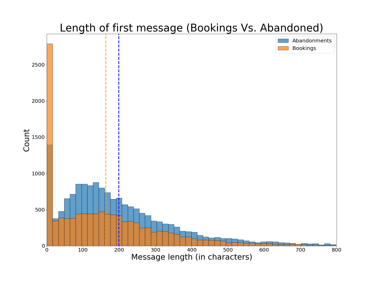
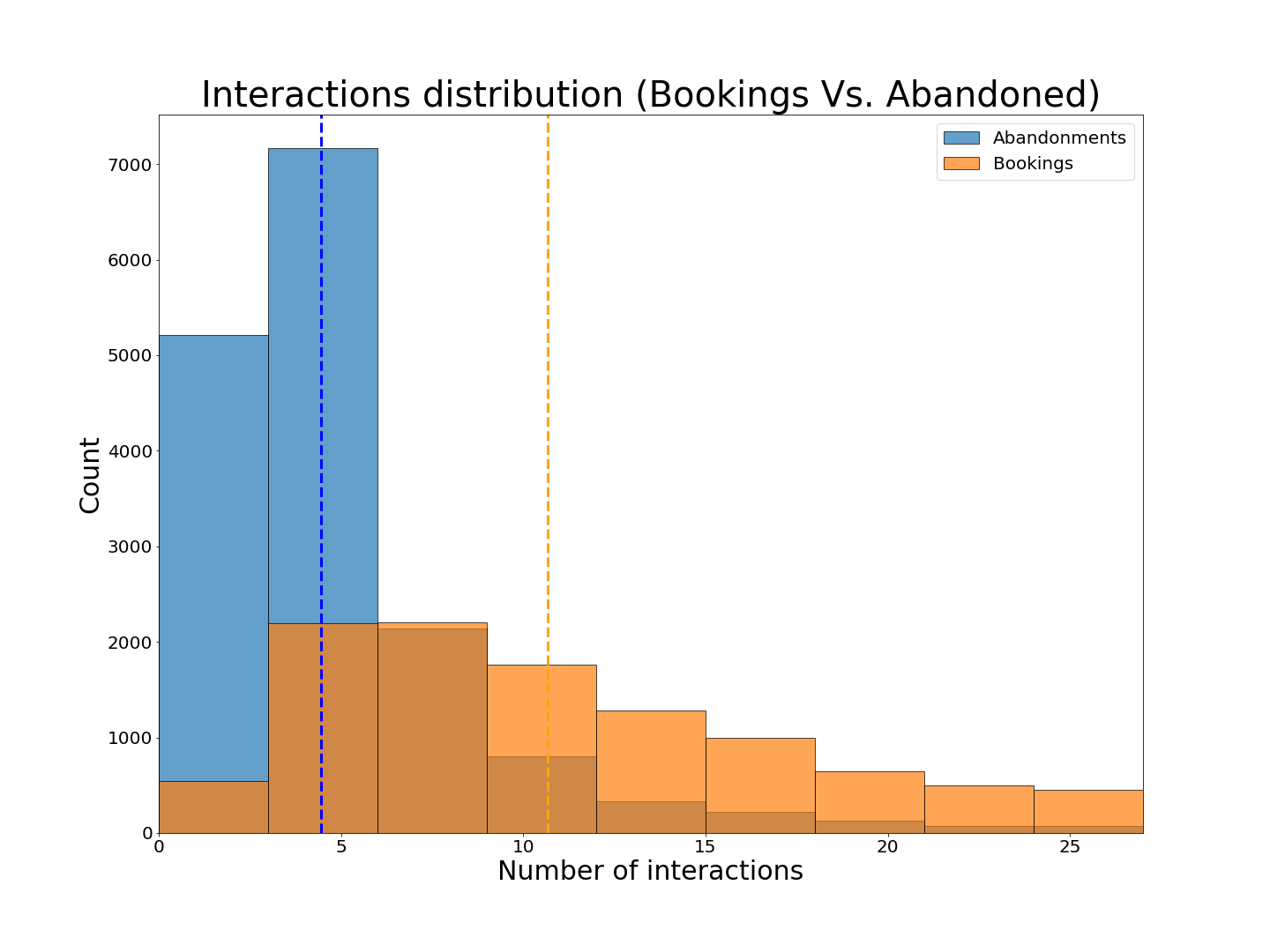
The following distributions plots provide further evidence to come up with measures to improve engagement.

To make a good first impression, the opening message should have no more than ~180 characters.
Also all the successful bookings have shown little over 10 interactions.

"Contact_me" performs poorly

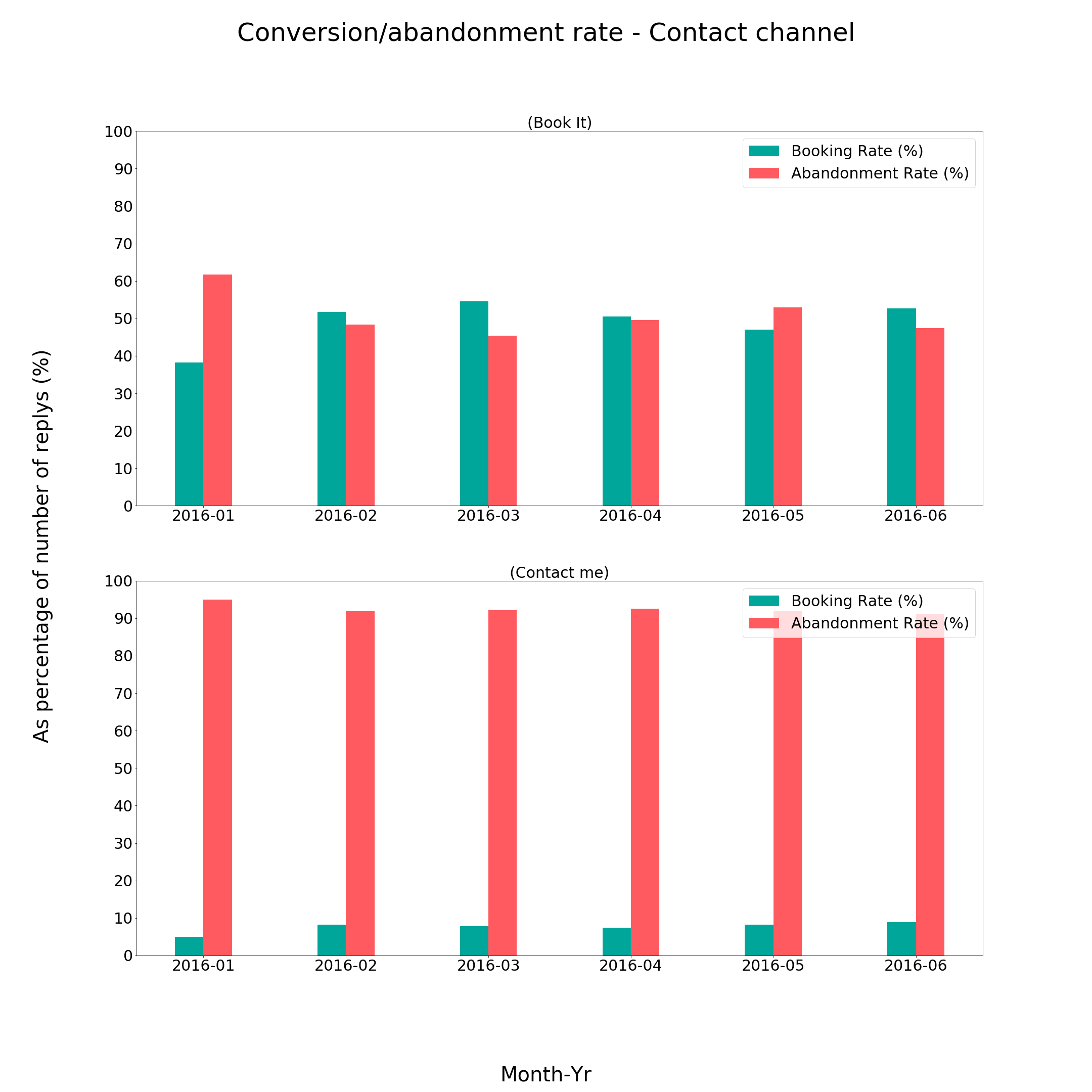
Looking at the abandonment rate in the figure below, we see that "Contact_me" channel type has 10 times the abandonment rate as compared to "book_it".

Note: The abandonment rate is a percentage of the total number of interactions started.

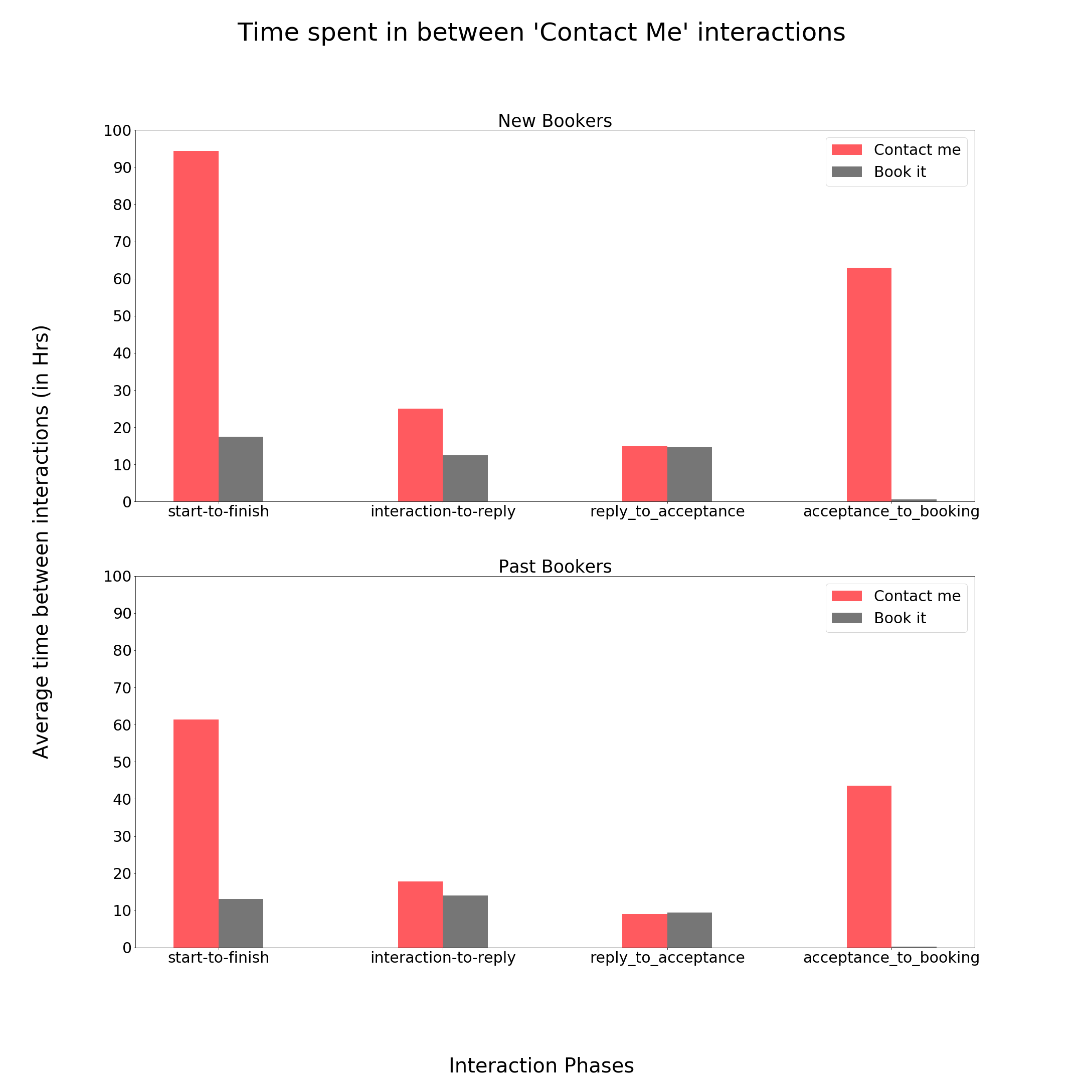
Digging a bit deeper, the following plot shows the time spent in number of hours between different phases of the interaction for new vs. returning buyers. We clearly see that average time for "Contact_me" between the phases is well over a day for both types of buyers, which provides further evidence against the channel.

2. Buildzoom - Top

Code Link

2.1 Problem Statement

Buildzoom gets data on building permits and wants to build a classifier that can correctly identify of the permit. The permit maybe of several types, but Buildzoom, wants a binary classification that can identify if a permit is (ELECTRICAL/NON-ELECTRICAL).

2.2 Input Data

Data Column	Description
License Type	Types of license associated with the property (Electrical contractor license, Speciality contractor license)
Business Name	Name of business
Legal Description	Legal address/block information
Description	describes work that need to be done eg: Install low voltage security system
Type (y)	ELECTRICAL/NON-ELECTRICAL
Subtype	Commercial/Single Family
Job Value	Value associated with the job

2.3 Technologies

Python libraries: Pandas, NumPy, Scikit-learn, NLTK, XGBoost, Regex

EDA Code
Machine Learning Code

2.4 References

StatQuest: https://www.youtube.com/watch?v=GrJP9FLV3FE&t=2217s
Data School: https://www.youtube.com/watch?v=irHhDMbw3xo&t=135s

3. DataRobot - Top

Code Link

3.1 Problem Statement

DataRobot wants to build a classification model to predict if an applicant is going to default on loan or not. Which loan applicants are most profitable and worthy of lending money to?

Following snippet of code shows the data dictionary. is_bad is the binary classification variable we want to predict. Based on some EDA the data set is highly imbalanced, so we need to make sure that we are using evaluation metrics that accounts for it.

3.2 Data

import pandas as pd

data_dict = pd.read_csv('/datarobot/data/data_dictionary.csv')
print(data_dict)

Index	Column Name	Type	Description	Category
0	addr_state	Categorical	Customer State	Customer
1	annual_inc	Numeric	Annual Income	Customer
2	collections_12_mths_ex_med	Numeric	(Credit based)	Customer
3	debt-to-income	Numeric	Ratio of debt to income	Loan
4	delinq_2yrs	Numeric	Any delinquency in last 2 years	Customer
5	earliest_cr_line	Date	First credit date	Customer
6	emp_length	Numeric	Length in current job	Customer
7	emp_title	Text	Employee Title	Customer
8	home_ownership	Categorical	Housing Status	Customer
9	Id	Numeric	Sequential number	Identifier
10	initial_list_status	Categorical	Loan status	Loan
11	inq_last_6mths	Numeric	Number of inquiries	Customer
12	is_bad	Numeric	1 or 0	Target
13	mths_since_last_delinq	Numeric	Months since last delinquency	Customer
14	mths_since_last_major_derog	Numeric	(Credit based)	Customer
15	mths_since_last_record	Numeric	Months since last record	Customer
16	Notes	Text	Notes taken by the administrator	Loan
17	open_acc	Numeric	(Credit based)	Customer
18	pymnt_plan	Categorical	Current Payment Plans	Customer
19	policy_code	Categorical	Loan type	Loan
20	pub_rec	Numeric	(Credit based)	Customer
21	purpose	Text	Purpose for the loan	Loan
22	purpose_cat	Categorical	Purpose category for the loan	Loan
23	revol_bal	Numeric	(Credit based)	Customer
24	revol_util	Numeric	(Credit based)	Customer
25	total_acc	Numeric	(Credit based)	Customer
26	verification_status	Categorical	Income Verified	Loan
27	zip_code	Categorical	Customer zip code	Customer

3.3 Feature Engineering

3.3.1 Numeric Data

For numeric data the missing values were replaced/imputed by the most occurring value or the mean() if the count of missing value was <1% and feature scaling was performed using the minmaxscaler() method of sklearn library.

3.3.2 Categorical Data

For categorical data missing values were replaced by "None". If a particular feature had too many categories, they were grouped together into broader categories. For eg: emp_title or Employer title feature had names of employers appering in different patterns.

Following are different patterns in which the US Army, the US Navy and Walmart appeared in. These varied appearence were replace with the more common 'U.S. Army', 'U.S. Navy', 'Walmart'

US Army patterns: ['U.S. Army', 'US Army', 'US ARMY', 'United States Army', 'us army', 'US Army', 'United States Army', 'US military army', 'united states army', 'U.S. Army', 'united States Army', 'US Army', 'U.S army', 'Us Army', 'U.S Army', 'U. S. Army', 'Us army']

US Navy patterns: ['US Navy', 'U.S. Navy', 'US Navy', 'US NAVY', 'Us Navy', 'United States Navy']

Walmart patterns: ['Wal-Mart', 'WAL-MART', 'Walmart', 'WalMart', 'wal-mart', 'walmart']

Some categorical features were biased towards one category 99:1 so they were dropped, because they weren't predictive of is_bad the target variable.

Date variable had information dated as early as 1960's. So they were replaced with quarter and year as two separate variables.

3.3.3 Text Data

For text data i.e. Notes in the feature engineering stage, NLTK was used to remove stop words and special characters from the notes from potential loan applicants. Stemming and Lemmatizers were applied, but the results with the ML model weren't great so they were skipped.

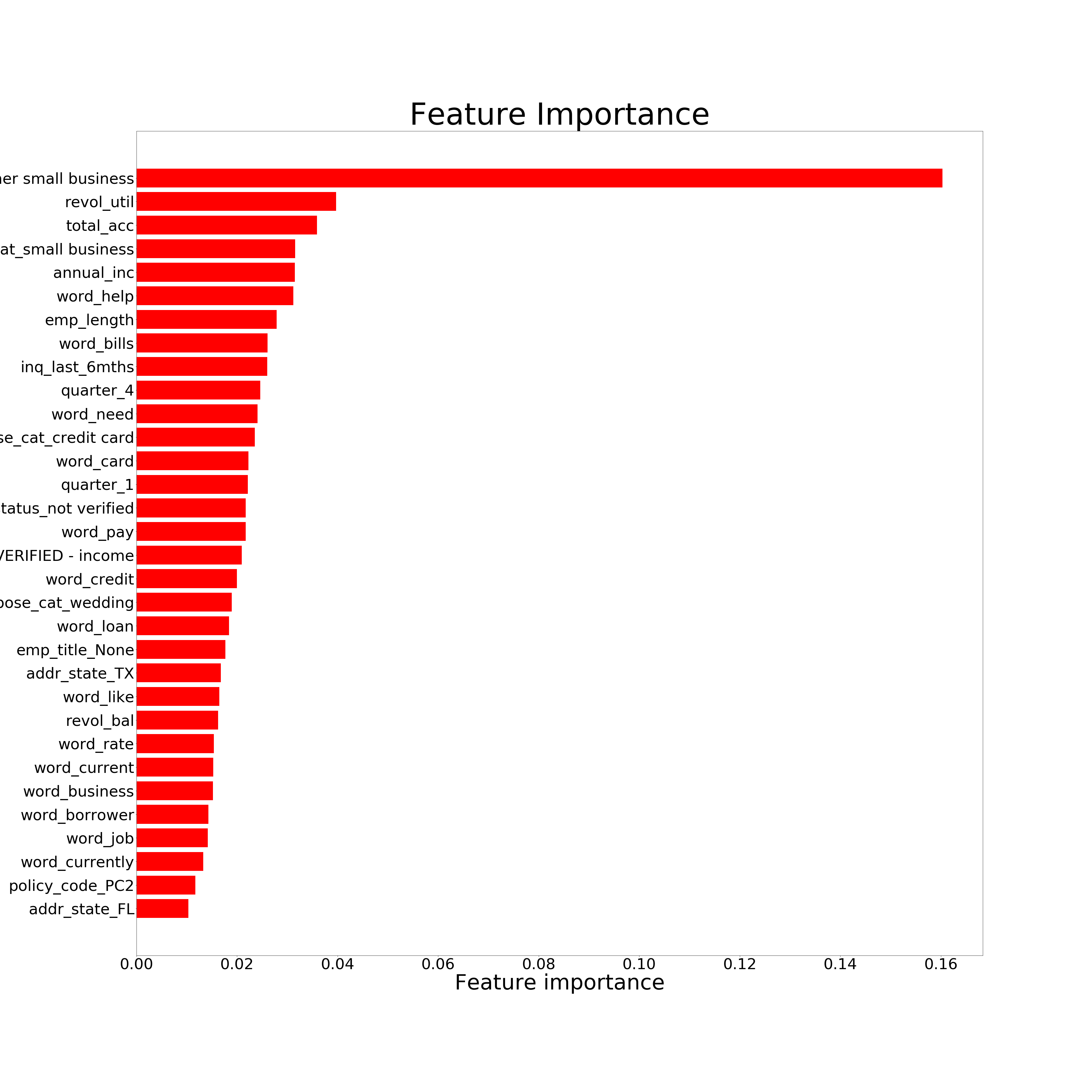
Further tfidf_vectorizer() from sklearn was used to encode text features into numeric one's. Following were the keywords that were more important in categorizing the target variable is_bad:

Important keywords: bills, borrower, business, card, credit, current, currently, help, job, like, loan, need, pay, rate

3.4 Machine Learning Model

3.4.1 XGBoost

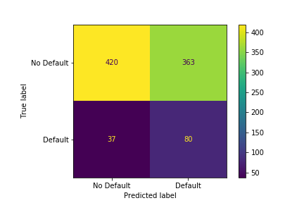
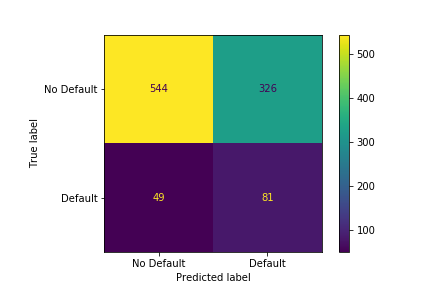
XGBoost model was trained to maximize sensitivity/recall for prediction, because of all the one's that defaulted we want the capacity to predict most of them ~70% or higher prediction accuracy.

After performing Grid search for hyper-parameter tuning and some amount of manual tuning, we get the following confusion matrix for our validation and test set.


Figure 1: Validation set - Confusion matrix


Figure 2: Test set - Confusion matrix

We also need to figure out the set of features that are predictive of our target variable i.e is_bad.


Figure 3: Feature Importance

NikhilSawal/data_science_case_studies