This tutorial describes the data and analysis considered for Bayesian hierachical model for Regional flood frequency analysis.
First, you need to install the SpatGEVBMA package from NorskRegnesentral GitHub respository
# install.packages("devtools")
devtools::install_github("NorskRegnesentral/SpatGEVBMA")
Then load the data and functions used for the analysis.
# Load yearly flood time series and covariates
load("~/BRFFA/data/norwayFlood.Rdata")

# Load functions
source('~/BRFFA/scripts/functions.R')
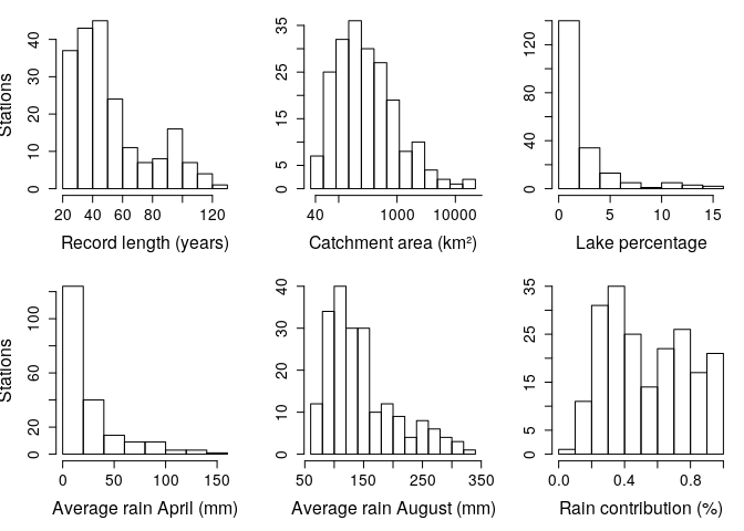
We start by exploring some descriptive plots of the covariates. Considering first histograms of the record length, catchment area, percentage of lake, average rain in April and August and percentage of flood contributed to rain vs. snowmelt.
# Define location for map plotting
S <- cbind(covariates$longitude,covariates$latitude)

#Plot histograms for some covariates
par(mar=c(5,4,1,1),mfrow=c(2,3),cex.axis=1.3,cex.lab=1.5)
hist(rowSums(!is.na(floodData)),xlab='Record length (years)',ylab='Stations',main = '')
hist(log(covariates$area.total),xlab='Catchment area (km²)',ylab='',main = '',xaxt='n')
axis(1,at=log(c(40,10^(2:6))),labels=c(40,10^(2:6)))
hist(covariates$pct.eff.lake,xlab='Lake percentage',ylab='',main = '')
hist(covariates$avg.rain.april,xlab='Average rain April (mm)',ylab='Stations',main = '')
hist(covariates$avg.rain.august,xlab='Average rain August (mm)',ylab='',main = '')
hist(covariates$avg.frac.rain,xlab='Rain contribution (%)',ylab='',main = '')
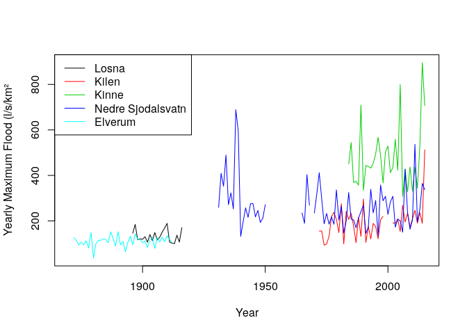
Now we plot the time series of some selected stations.
matplot(1870:2015,t(floodData[c(7,50,80,2,23),])*1000,type='l',lty=1,xlab='Year',ylab = 'Yearly Maximum Flood (l/s/km²')
legend('topleft',lty=1,col=1:5,legend=covariates$station.name[c(7,50,80,2,23)])
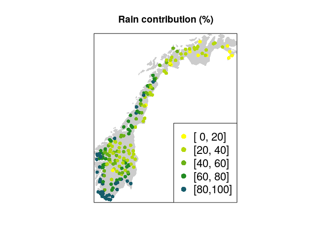
Then we plot the percentage of flood contributed to rain vs. snowmelt according to longitude and latitude of the each considered station, to reveal the spatial distribution of this covariate.
#Plot map for some covariates
library(maps)
all.colors <- colorRampPalette(c("yellow","forestgreen", "blue"))(7) #heat.colors(7)[7:1]
par(mar=c(5,4,1,1),mfrow=c(1,1))
var1 <- covariates$avg.frac.rain
mugr <- rep(NA,length(var1))
gr <- seq(0, 1, length.out=6)
#gr <- c(0,0.1,0.2,0.3,0.5,0.7,1)
for (g in 1:(length(gr)-1)){
  mugr[var1>=gr[g] & var1<gr[g+1]] <- g
}
gr <- 100*gr
ltxt <-  paste0("[",format(gr[-length(gr)]),",",format(gr[-1]),']') # text for legend

par(mar=c(0,0,3,0))
maps::map("world",regions="Norway",fill=TRUE,col="gray80",ylim=c(58,71),xlim=c(5,30.5),border=FALSE)
title("Rain contribution (%)")
box()
points(S[,1], S[,2], pch=16, col=all.colors[mugr])
legend("bottomright",legend=ltxt,fill=,col=all.colors[1:7],pch=16,cex=1.4)The main analysis is carried by running 100 000 MCMC simulation by the SpatGEV package. The flood data is structured as a list of time series, one for each station, to allow for difference serie lengths. The covariates are centered and scaled before analysis.
###
# set the response variable
####
#datalist <- as.list(as.data.frame(t(floodData/covariates$area_total)))
datalist <- as.list(as.data.frame(t(floodData)))
# remove all NA's from datalist
for (i in 1:length(datalist)) {
  datalist[[i]] <- (datalist[[i]])[!is.na(datalist[[i]])]
}

#Construct matrix of covariates
covMat <- as.matrix(covariates[,2:13])

# Standardize covariates
for (i in 2:dim(covMat)[2]) {
  covMat[,i] <- standardiseVar(covMat[,i])
}

# Add intercept
covMat <- cbind('Constant' = rep(1,dim(covMat)[1]),covMat)

# Specify prior
prior.user <- NULL
prior.user$eta$beta.0 <- c(log(1000),rep(0,dim(covMat)[2]-1))
First, the SpatGEVBMA package is loaded. We run the package with the options to to non-spationally distributed error, to have the regression model for the scale parameter on a log scale and to print an output for every 5000 MCMC run.
In the paper, Bayesian Regional Flood Frequency Analysis for Large Catchments we use 100 000 simulations, but in the following we demonstrate the code by running 100 simulations.
library(SpatGEVBMA)
nsim <- 100
res <- spatial.gev.bma(datalist,covMat,S,nsim,prior.user=prior.user,
                       nonspatial = TRUE, log.kappa=TRUE,print.every=5000)
res$cov.names <- colnames(covMat)
The result can be analysed by first removing a suitable range of burn-in samples, we seletion 20 000 or 20% of the total MCMC runs. The calculated the inclustion probabilities for each of the covariates within the location (\mu), scale (\log\kappa), and shape (\xi) parameter of the GEV distribution.
##                     mu kappa  xi
## Constant           100   100 100
## longitude            0    62   0
## latitude             0    86   1
## pct.eff.lake        79   100   0
## inflow               0    19  30
## avg.frac.rain        0    89   0
## area.total           0    29   0
## avg.rain.april     100    24   0
## avg.rain.august    100   100   6
## avg.snowmelt.march   0    14   0
## gradient            91    28   0
## pct.bedrock        100    32   0
## relative.area        0    91   0
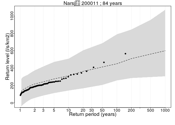
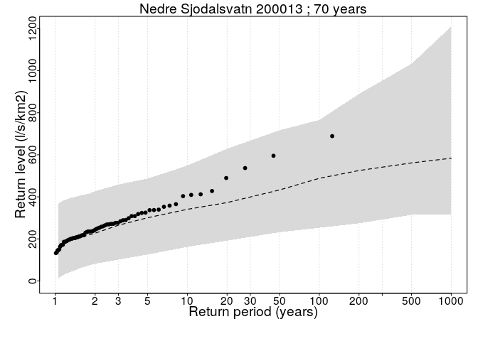
Then we plot the resulting distribution according to the quantiles or return values, e.g for 1000 year flood, we calculated the (1 - 1/1000 = 0.999) quantile. The random effects for each MCMC run are simulated from a Gaussian distribution with the corresponding variance (1/\alpha^{(r)}), separately for each distribution parameter.
##########################################
###### #Plot return values plots
##########################################

#Selection of station
st.no <- rownames(floodData)[1:2]
T <- c(seq(1.05,1.9,by=0.05),2,3,5,10,20,50,100,200,500,1000)
return.level <- list()
len <- dim(res$THETA[-(1:burn),,])[1] #len=nsim-burn
zp <- matrix(0,nrow=len,ncol=length(T))
p <- 1/T

# Calculated GEV distribution based on MCMC samples
for (i in st.no) {
  mu <- res$THETA[-(1:burn),,1]%*%covMat[i,] + rnorm(len,0,sd = 1/sqrt(res$ALPHA[-(1:burn),1]))
  ka <- res$THETA[-(1:burn),,2]%*%covMat[i,] + rnorm(len,0,sd = 1/sqrt(res$ALPHA[-(1:burn),2]))
  xi <- res$THETA[-(1:burn),,3]%*%covMat[i,] + rnorm(len,0,sd = 1/sqrt(res$ALPHA[-(1:burn),3]))
  if(res$log.kappa) ka <- exp(ka)
  for(j in 1:length(T)) {
    zp[,j] <- returnLevel(mu,ka,xi,T[j],useGumbel=FALSE)
  }

  tmplist <- list()
  tmplist$MEAN <- apply(zp,2,median)
  tmplist$lower <- apply(zp,2,quantile,0.1)
  tmplist$upper <- apply(zp,2,quantile,0.9)
  return.level[[i]] <- tmplist
}

#Plot return values plots
plotReturnLevel(return.level = return.level,floodData = floodData,
                floodCov = covariates,
                T=T,writeToFile=FALSE,ymin=-0.01,ymax=NULL)
## [1] "200011" "200013"
