The networkR package provides a set of functions for the analysis of social and economic networks and hypergraphs. As such, the package provides a range of tools to analyse both the macroscopic and microscopic features of networked systems. The macroscopic analysis include the degree distribution, diameter and density of the network. The microscopic analysis includes the power, influence and centrality of individual nodes.
The primary use of the package is the analysis of social and economic networks; including directorate networks that are represented as hypergraphs.
No versions have been officially released yet. Currently we are still beta testing and adding new functionality, however we will post any new versions here when realeased.
There is no CRAN version available yet. Instead, consider the following installation instructions for devtools.
# install.packages("devtools")
library(devtools)
devtools::install_github("O1sims/networkR")
The package also contains empirical and synthetic data. This is supplied to allow for testing of the package. As we are dealing with network data we partition the dataset into a nodeList and an edgeList. If we are dealing with a hypergraph we also include an affiliationList to the dataset. The functions typically require these data components.
The package provides four empirical network and hypergraph datasets.
Florentine marriages: The first network dataset is the elite marriage network of Renaissance Florence circa 1435. This dataset has been used in various representations in a number of network-oriented academic articles. The data was originally sourced from Padgett and Ansell (1994). The static network consists of 32 families and 31 arcs, meaning that a number of families are singletons. Arguably these nodes could be disregarded from the analysis.
- Marriage Data:
florentineNodes.rdaandflorentineEdges.rda.
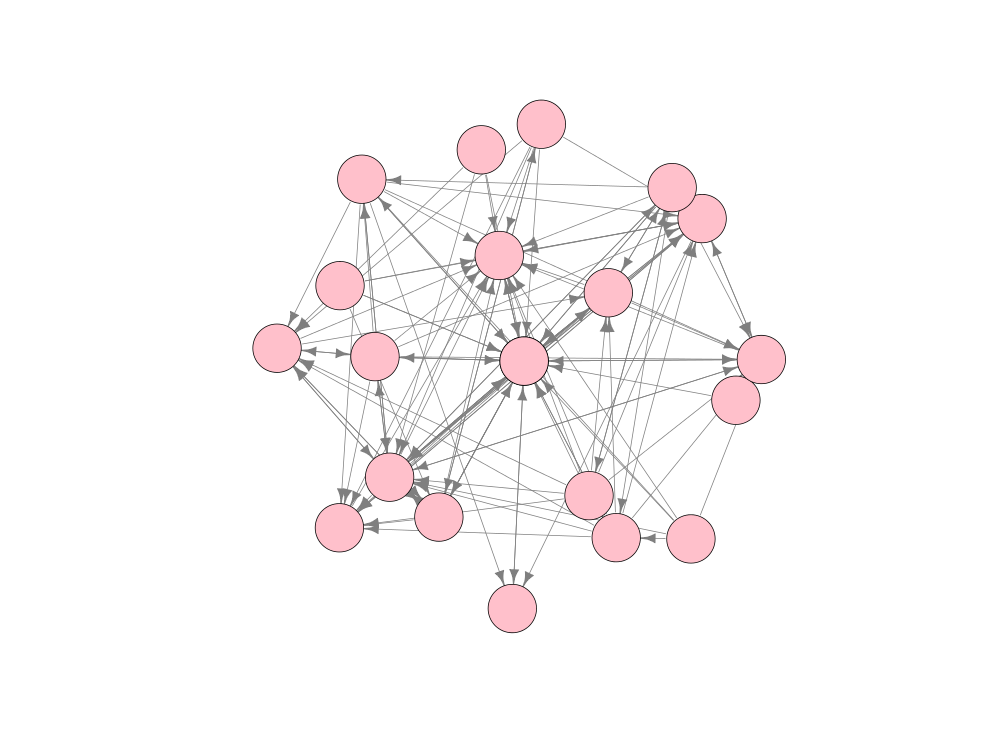
Manager advice: The second network dataset is the manager advice network gathered by David Krackhardt (1987). This directed network contains 21 managers from 4 different levels of management and also contains 129 arcs between the managers.
- Advice data:
managerNodes.rdaandmanagerEdges.rda.
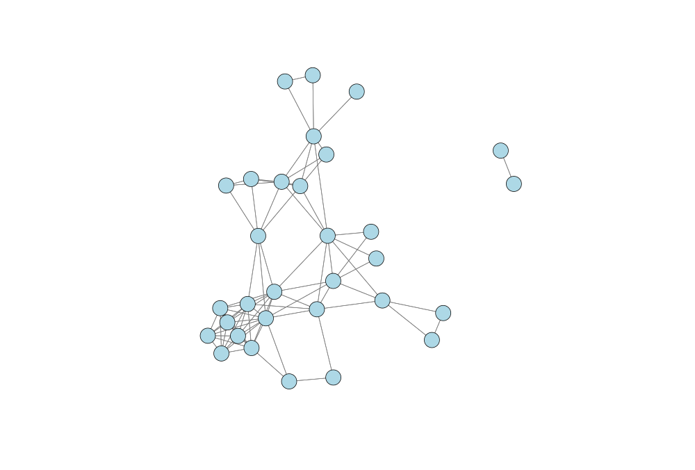
9/11 terrorists: The third dataset refers to four different networks that show the evolution of the interactions between terrorists that coordinated and instigated the 9/11 terrorists attacks. These networks span from December 1999 to August 2001, just before the attack. The size of the network increases over time from 27 terrorists in December 1999 to 32 terrorists in August 2001. The network also becomes more concentrated over time. These networks have been constructed from a number of different sources within academic literature, government reports and journalist articles.
- Terrorist data:
terroristNodes.rdaandterroristEdges.rda.
Directors of New York City: The final dataset refers to a hypergraph representing the directorate of New York City in 1902. We provide a bipartite network of all railways, insurance, and financial institutions as well as their directors. The purpose of this data is to illustrate the control of directors and firms in New York during this time. This network contains over 250 unique firms and 3000 unique directors. There are 4299 links; each link indicates membership of a director to a firm. Since the number of links is greater than the number of unique directors it is certain that overlapping directorate exists. This network has been constructed from historical New York Times articles and the Directory of Directors of New York City. Other sources are used to acquire data on the valuation of each of the firms.
- Directorate data:
nycNodes.rda,nycAffiliations.rdaandnycHypergraph.rda.
A number of example or test data are provided. These can be used to test the functions within the package.
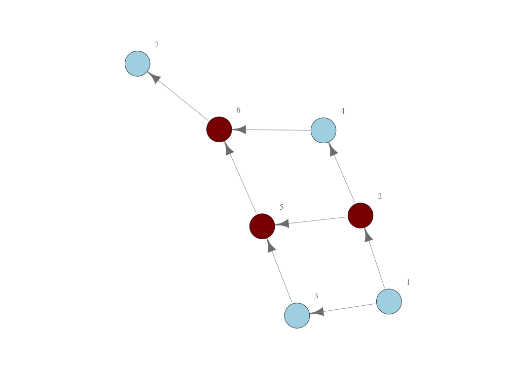
Consider the directed network in network1Nodes.rda and network1Edges.rda. The network contains 7 nodes---one of which is a source and another is a sink---and 8 arcs that can be interpreted as the flow of information, money, or economic goods: node 1 is connected to node 7 through the intermediation of other nodes in the network. The network of relationships is plotted in the Figure below.
Let's look at a number of networkR functions applied to the first test network (network1Nodes.rda and network1Edges.rda). Load these files up.
> library(networkR)
> data(list = c("network1Nodes", "network1Edges"))
It is pretty obvious from reviewing this network that nodes 2, 5, and 6 are all middlemen. Furthermore, it is noticeable that node 6 would still remain a middleman regardless of whether the network were transformed into its undirected state. We get the following values when running the middlemanPowerDetail() function.
> middlemanPowerDetail(network1Edges, network1Nodes)
number name power normPower        		type
	 1    1     0       0.0    Non-middleman
	 2    2     1       0.1   Weak middleman
	 3    3     0       0.0    Non-middleman
	 4    4     0       0.0    Non-middleman
	 5    5     2       0.2   Weak middleman
	 6    6     5       0.5 Strong middleman
	 7    7     0       0.0    Non-middleman
As hypothesised we find that nodes 2 and 5 are both weak middlemen and node 6 is a strong middleman. To add to this we also find : (a) the number of relationships brokered by all middleman, and (b) the normalised middleman power for each node. We can represent middlemen visually with the following R commands:
> colourMiddlemen <- middlemanPowerDetail(network1Edges, network1Nodes)
> colourMiddlemen$colour <- ifelse(colourMiddlemen$power > 0, "darkred", "lightblue")
> isTrue <- isUndirected(network1Edges, network1Nodes) == FALSE
> plot(graph_from_data_frame(network1Edges,
							 directed = isTrue),
	   vertex.color = middle$colour,
	   vertex.label.dist = 3,
	   vertex.size = 20,
	   edge.color = "gray50")
In this case, the network is plotted such that middlemen are coloured in red and non-middlemen are coloured in blue. This is seen in the Figure below.
The coverage of each node set in the 7 node network is given by:
> setCoverage(network1Edges, network1Nodes)
		 set setSize  successors predecessors noSucc noPred coverage
1:         1       1 2,3,4,5,6,7            0      6      0        0
2:         2       1     4,5,6,7            1      4      1        4
3:         3       1       5,6,7            1      3      1        3
4:         4       1         6,7          1,2      2      2        4
5:         5       1         6,7        1,2,3      2      3        6
---
115: 2,3,4,5,7     5           6          1,6      1      2        1
116: 2,3,4,6,7     5           5          1,5      1      2        1
117: 2,3,5,6,7     5           4          1,4      1      2        1
118: 2,4,5,6,7     5                      1,3      0      2        0
119: 3,4,5,6,7     5                      1,2      0      2        0
The brokerage, or middleman power, of each node set can be derived in much the same way. This is done by executing the setBrokerage() function. We arrive at the following output:
> setBrokerage(network1Edges, network1Nodes)
		 set setSize  successors predecessors noSucc noPred power
1:         1       1 2,3,4,5,6,7            0      6      0     0
2:         2       1     4,5,6,7            1      4      1     1
3:         3       1       5,6,7            1      3      1     0
4:         4       1         6,7          1,2      2      2     0
5:         5       1         6,7        1,2,3      2      3     2
---
115: 2,3,4,5,7     5           6          1,6      1      2     1
116: 2,3,4,6,7     5           5          1,5      1      2     1
117: 2,3,5,6,7     5           4          1,4      1      2     1
118: 2,4,5,6,7     5                      1,3      0      2     0
119: 3,4,5,6,7     5                      1,2      0      2     0
We can see that a positive coverage does not translate to a positive middleman power. More specifically, the middleman power of a node set is defined on the critical sets of the network. All critical sets are provided with the function criticalSets(). The output for the 7 node network is as below:
> criticalSets(network1Edges, network1Nodes)
		 set setSize successors predecessors noSucc noPred power powerCapita
1:         2       1    4,5,6,7            1      4      1     1       1.000
2:         5       1        6,7        1,2,3      2      3     2       2.000
3:         6       1          7    1,2,3,4,5      1      5     5       5.000
4:       1,5       2  2,3,4,6,7          2,3      5      2     2       1.000
5:       1,6       2  2,3,4,5,7      2,3,4,5      5      4     4       2.000
---
62: 1,3,4,5,7      5        2,6          2,6      2      2     1       0.200
63: 2,3,4,5,6      5          7            1      1      1     1       0.200
64: 2,3,4,5,7      5          6          1,6      1      2     1       0.200
65: 2,3,4,6,7      5          5          1,5      1      2     1       0.200
66: 2,3,5,6,7      5          4          1,4      1      2     1       0.200
This function also provides the middleman power per capita.
The criticality of individual or sets of nodes is a measure of their assumed brokerage after they have been allowed the ability to form coalitions and actively broker relations. It is therefore a measure based on the resulting stable sets. We use the notion of Strong Nash equilibrium (SNE) to determine the stability of a coalition within a network. Each coalition also has some cost of formation; this cost function can also be determined within the model itself.
For example, when considering the network of 7 nodes when there exists no costs in forming blocks we can determine the SNE as follows:
> blockSNE(network1Edges, network1Nodes)
   set setSize successors predecessors noSucc noPred power powerCapita
1:   6       1          7    1,2,3,4,5      1      5     5           5
2: 4,5       2        6,7        1,2,3      2      3     6           3
3: 2,3       2    4,5,6,7            1      4      1     4           2
Specifically, node 6 remains as a middleman and two blocks are formed: one containing nodes 4 and 5, and another containing nodes 2 and 3. All other nodes do not form a block and therefore earn a payoff of zero. If, however, there is some substantial cost of forming a block, then the SNE degredates to the point where no blocks are formed and middlemen are the only nodes that earn a positive payoff. By setting c = 2 we get the following Strong Nash equilibrium:
> blockSNE(network1Edges, network1Nodes, c = 2)
   set setSize successors predecessors noSucc noPred power powerCapita
1:   6       1          7    1,2,3,4,5      1      5     5           5
2:   5       1        6,7        1,2,3      2      3     2           2
3:   2       1    4,5,6,7            1      4      1     1           1
The criticality of individual nodes can be calculated from all potential SNE blocks that are known the emerge. Simply, the criticality of all nodes in the network is calculated as:
> nodeNormCriticality(network1Edges, network1Nodes)
[1] 0.0 0.2 0.2 0.3 0.3 0.5 0.0
A set of functions for analysing hypergraphs are provided in the package. These functions revolve around the projection of hypergraphs into different network structures and the measurement of a node or an affiiations "control" within the hypergraph. This notion of control as a centrality measure is represented by the sigma score and beta measures within hypergraphs. Within the realm of socio-economic networks, the best application of hypergraphs come in the form of corporate directorate networks.
Two such examples are provided in the dataset alongside this package:
- New York City (NYC) corporate directors of 1902; and
- The corporate directors of Victorian Britain between 1880 and 1900.
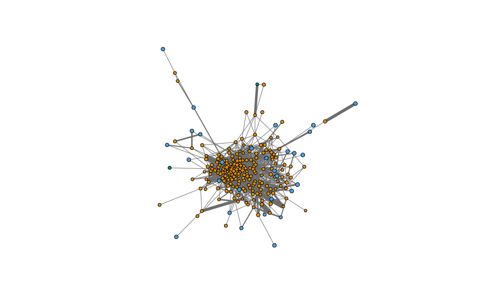
NYC corporate directors: Using the NYC Directorate data (1902) we can illustrate an example of an affiliation projection of the directorate hypergraph. Consider the following code.
> c("nycNodes", "nycAffiliations", "nycHypergraph") %>% data()
> projection <- nycHypergraph %>%
affiliationProjection() %>%
filterNetwork()
> plot(graph_from_data_frame(projection,
                             directed = FALSE),
        vertex.color = nycAffiliations$types,
        vertex.label = NA,
        vertex.label.dist = 3,
        vertex.label.color = "black",
        vertex.size = log(nycAffiliations$valuations)/5,
        edge.width = projection$weight,
        edge.color = "grey50",
        edge.arrow.size = 0)
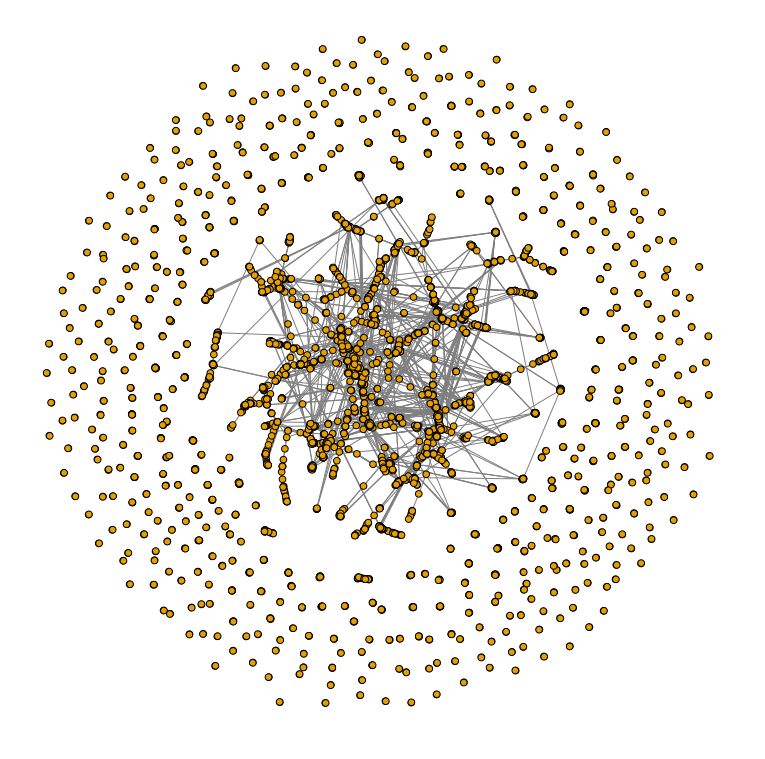
Victorian Britain directors: The Victorian Britain directorate data (1880-1900), which can be found in its raw format here, can also be used in much the same way. See the code below:
> data(list = c("vbdNodes", "vbdAffiliations", "vbdHypergraph"))
> projection <- vbdHypergraph %>%
    affiliationProjection() %>%
    filterNetwork()
> plot(graph_from_data_frame(
    projection,
    directed = FALSE),
    vertex.label = NA,
    vertex.label.dist = 3,
    vertex.label.color = "black",
    vertex.size = 2,
    edge.width = projection$weight,
    edge.color = "grey50",
    edge.arrow.size = 0)
This generates the following institutional overlap for firms in 1880.
It is important to understand the structure of the hypergraph data that needs to be passed to the functions. Data is structured such that a bipartite network is expressed: nodes are connected to affiliations by an edge, however a set of nodes nor a set of affiliations are connected to each other directly.
Affiliations within a hypergraph can be associated within an "aspect". As such, an affiliation can be associated with one and only one affiliation. We consider these cases and discuss the analysis and formation of elite networks in aspectual hypergraphs.
For example, when analysing director networks each firm exists within one industry and therefore one aspect of the economy. An elite director is one who is on the board of companies of every industry under analysis.
> data(list = c("nycNodes", "nycAffiliations", "nycHypergraph"))
> elites(nycHypergraph, nycNodes, nycAffiliations, nycAffiliations$types)
       number                nodes
  1:      212        JAMES H. HYDE
  2:      220        E.H. HARRIMAN
  3:      240    SAMUEL D. BABCOCK
  4:      268      GEORGE F. BAKER
  5:      272     JOHN JACOB ASTOR
  ---
  31:    1886      GEORGE J. GOULD
  32:    1956         BRAYTON IVES
  33:    2131      STUYVESANT FISH
  34:    2679 N. PARKER SHORTRIDGE
  35:    2907      JACOB H. SCHIFF
All directors listed were seen as influential during this time period.
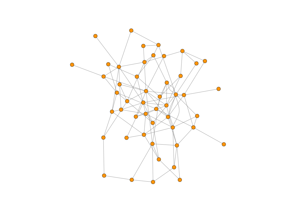
A number of other functions are defined in networkFunctions.R. For example, the randomGraph() function provides an Erdos-Renyi graph where the probability of an arc or link existing between any two nodes is explicitly defined within the argument 0 < p < 1.
> erdosRenyi <- randomGraph(
    n = 50,
    p = 0.05)
> plot(graph_from_data_frame(
    erdosRenyi,
  directed = FALSE),
	  vertex.color = "orange",
	  vertex.label = NA,
	  vertex.label.dist = 3,
	  vertex.size = 5,
	  edge.color = "gray50",
	  edge.arrow.size = 0)
This generates the following graph:
