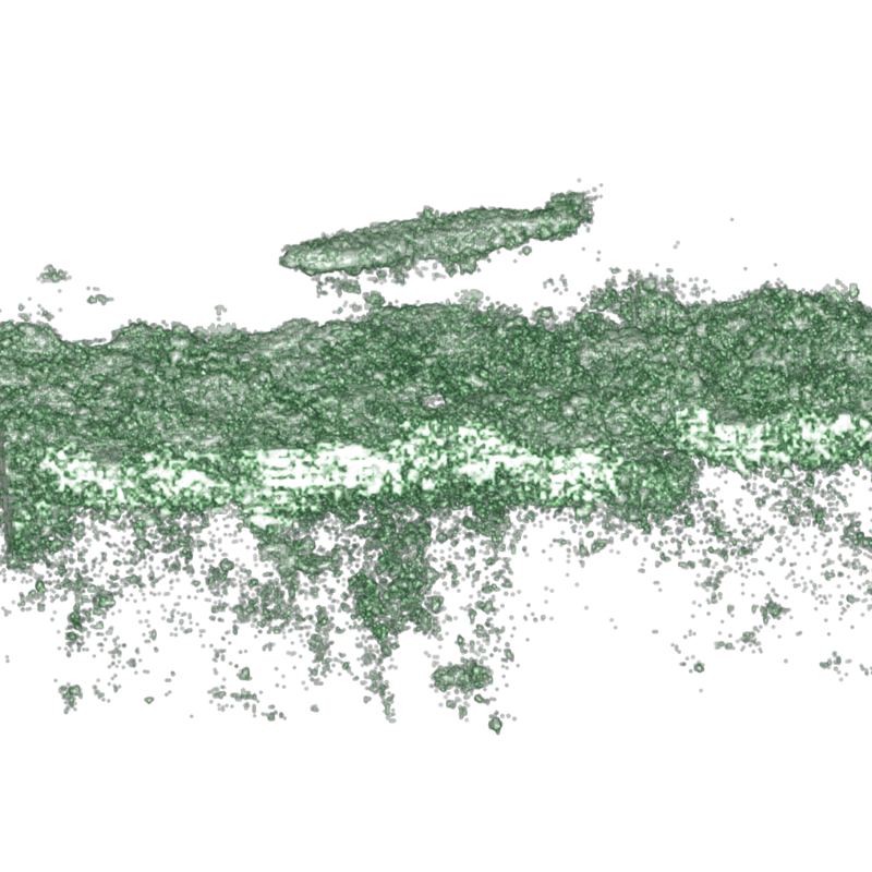
Codebase for Neural Volumetric Reconstructions for Coherent Synthetic Aperture Sonar by Albert W. Reed, Juhyeon Kim, Thomas Blanford, Adithya Pediredla, Daniel C. Brown, and Suren Jayasuriya.
We have tested the code on an A100 GPU, 3080 GPU, and 3090 TI GPU. The GPU will need at least 7GB of VRAM. We provide scripts for reconstructing the scenes with low and higher memory settings (see section Reconstruct the armadillo using backprojection and our method for more details).
Some of the code uses QT libraries which require the libxcb-cursor0 to be installed via:
sudo apt-get update -y
sudo apt-get install -y libxcb-cursor0
In the paper, we render the reconstruct results using Matlab. The matlab scripts in this repo were tested on Matlab 2023b. Some of the syntax may not be compatible with older Matlab versions.
git clone https://github.com/awreed/Neural-Volumetric-Reconstruction-for-Coherent-SAS
cd Neural-Volumetric-Reconstruction-for-Coherent-SAS
Use the following commands for setting up the code environment. These commands were tested in a Linux environment with an A100 GPU.
conda create --name nvr_sas -y python=3.8
conda activate nvr_sas
python -m pip install --upgrade pip
Install PyTorch 2.0.1 with CUDA 11.8.
pip install torch==2.0.1+cu118 torchvision==0.15.2+cu118 --extra-index-url https://download.pytorch.org/whl/cu118
Install the tiny-cuda-nn dependencies used for the neural network.
conda install -c "nvidia/label/cuda-11.8.0" cuda-toolkit
pip install ninja git+https://github.com/NVlabs/tiny-cuda-nn/#subdirectory=bindings/torch
pip install -e .
You may skip this step if you prefer not to use tensorboard. You can start a
tensorboard session by running run_tensorboard.sh. You may populate the script with your details:
tensorboard --logdir ./ --host <host-number> --port <port-number>. Note that you may find <host-number> using the
hostname -I command on Ubuntu.
GRSI: For the sake of time, please skip this step by downloading the processed data directly in the Download the data section.
The following steps describe how to process the .csv files (e.g., Flight00000.csv) that are generated by
the AirSAS LabView code. The goal is to process the files into a data structure of tensors that we can use
with numpy/pytorch. This data structure is called a system_data.pik file, which
is a pickled python dictionary. At a high level, each scene has its own system_data.pik file (see Download the Data below)
which contains everything needed for reconstruction: the measurements, scene geometry, and other metadata (e.g., sound speed).
Download the airsas measurements for the bunny and armadillo:
gdown https://drive.google.com/uc?id=1mzJx_tesC3XDtUcnjrUvn11N2z8NuXEv
Unzip them using unzip or 7z:
unzip airsas_raw_data.zip
The unzipped data has the file structure
├── airsas_raw_data
│   ├── arma # AirSAS measurements of the armadillo
│   ├── background # AirSAS measurements of empty scene (used for background subtraction)
│   ├── bunny # AirSAS measurements of the bunny
.   .
.   .
.   .
Create system_data.pik file for the 20kHz armadillo using backproject_from_csv.sh as follows:
cd ./scenes/airsas/arma_20k
chmod +x backproject_from_csv.sh
./backproject_from_csv.sh <path/to/airsas_raw_data/arma> <path/to/airsas_raw_data/background> <output_dir>
A few things to note:
- The
backproject_from_csv.shscript populates the<output-dir>with the backprojected scene and create thesystem_data.pikfile that is necessary for our method in the next steps. - Notice that
backproject_from_csv.shcontains many commented parameters that can be changed to define the scene dimensions. For example, you could beamform a 2D scene by setting z_max = z_min and num_z = 1:-
# Modifying backproject_from_csv.sh to beamform a 2D scene on the z = 0 plane

python ../../../airsas/reconstruct_airsas_scene.py \
   .
   .
   .
   --z_min 0.00 `# Beamforming to the z = 0 plane`
   --z_max 0.00 `# Beamforming to the z = 0 plane`
   .
   .
   .
   --num_z 1 `# There is only "1" z voxel since it is a plane`
-
- The
system_data.pikcan be unpickled to recover a python dictionary. The dictionary structure adheres to the data schema defined inSASDataSchemaofdata_schemas.py.-
# You can unpickle and explore system_data.pik

import pickle
import constants as c

# unpickle the system_data.pik file
with open(system_data.pik, 'rb') as f:
      system_data = pickle.load(f) # system_data is a python dictionary

# For example, access the raw waveforms using
wfms = system_data[c.WFM_DATA]

# or the soundspeed using
sound_speed = system_data[c.sound_speed]

print(system_data.keys()) # This will print all the available keys. These are defined and commented in the SASDataSchema class in the file `data_schemas.py`
-
We can skip the next step (Download the data) since we created the pickle file from scratch.
Download the data:
gdown https://drive.google.com/uc?id=18yMVWS3ZxEgillaqs6aQXBnhgDcRD19c
Unzip the data:
unzip system_data_files.zip
to obtain: (1) system_data_bunny_20k.pik; (2) system_data_bunny_5k.pik; (3)system_data_arma_20k.pik;
(4) system_data_arma_5k.pik.
Each pickle files contain the data used to generate Figure 12 in the paper. The pickle files are named according to the scene (i.e., bunny or armadillo) and
which sonar waveform was used (i.e., 5k or 20k). Each pickle contains a python dictionary which holds the scene
geometry and measurements necessary for reconstruction.
We provide two reconstruction scripts for each AirSAS scene, one compatible for GPUs < 10GB and the other for GPUs > 20GB.
These are titled reconstruct_low_mem.sh and reconstruct_high_mem.sh, respectively. We have tested the reconstruct_low_mem.sh script on a 3080 GPU,
and the reconstrct_high_mem.sh on an A100. Note that we use reconstruct_high_mem.sh for the paper results. GPU usage
can be further reduced by lowering the max_weights in reconstruct_low_mem.sh, but reconstruction quality may be worse.
We will describe how to reconstruct the armadillo object measured with the 20kHz waveform. Note that reconstruct.sh
contains many hyperparameters that can be changed. Currently, they are set to the parameters used in the paper.
cd ./scenes/airsas/arma_20k
chmod +x reconstruct_low_mem.sh # or reconstruct_high_mem.sh if GPU has enough VRAM
./reconstruct_low_mem.sh <path/to/system_data_arma_20k.pik> <pick-an-experiment-name>
Successfully running the above will generate a new directory reconstructed_scenes/ populated with the backprojection result and our result:
├── scenes/airsas/arma_20k
│   ├── reconstructed_scenes
│        ├── backprojected_scene.mat # backprojected scene (h x w x d complex-valued)
│        ├── backprojected_scene.npy # npy version of backprojected scene
│        ├── final_upsampled_scene.mat # our reconstructed volumetric scene (h x w x d complex-valued)
│        ├── final_upsampled_scene.npy # npy version of our reconstructed scene
.   .
.   .
.   .
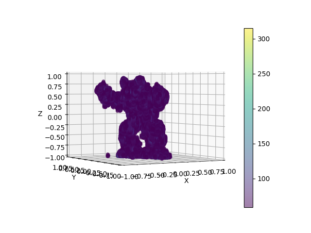
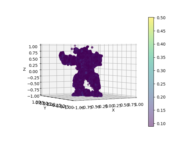
If we don't want to use Matlab, we can obtain quick (but poor) visualizations using Matplotlib.
Rendering the backprojection result (from the ./scenes/airsas/arma_20k directory):
python ../../../inr_reconstruction/matplotlib_render_cmd_line.py --scene_npy_file reconstructed_scenes/backprojected_scene.npy --output_dir ./reconstructed_scenes/ --output_name bp_mpl --thresh 3 --downsample_factor 1 --elev 2 --num_angles 4
Render our method's result:
python ../../../inr_reconstruction/matplotlib_render_cmd_line.py --scene_npy_file reconstructed_scenes/final_upsampled_scene.npy --output_dir ./reconstructed_scenes/ --output_name ours_mpl --thresh 3 --downsample_factor 2 --elev 2 --num_angles 4
The rendered images will be in scenes/airsas/arma_20k/reconstructed_scenes.
(left: backproject, right ours). See the Matlab section below for a better way to render the results.
We render the paper results using MATLAB's volshow() function. This requires access to a MATLAB installation that has the Imaging Processing Toolbox. Note that these results
could be rendered using any renderer we prefer --- they are simply complex-valued 3D (X x Y x Z) scenes. We take the abs() of the complex
scene before rendering to visualize the scene magnitude.
To render with matlab, navigate to the project's matlab directory :
cd Neural-Volumetric-Reconstruction-for-Coherent-SAS/matlab
This directory contains the function:
Syntax: volume_render_scene(scene_path, save_path, save_name, threshold, upsample_factor, colormap_option)
Parameters:
    scene_path: path to the *.mat file containing the scene
    save_path: path to save rendered image
    save_name: name to assign to rendered image
    threshold:  filter scene according to abs(scene) < threshold = 0
    upsample_factor: scaling factor for trilinearly upsampling the scene
    colormap_option: 0 for red, 1 for blue
    theta_in: rotation
    z: elevatation parameter
Render the backprojection result from a matlab terminal using
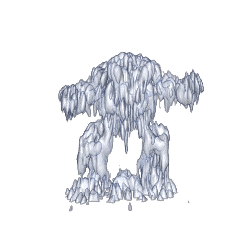
volume_render_scene('../scenes/airsas/arma_20k/reconstructed_scenes/backprojected_scene.mat', '../scenes/airsas/arma_20k/reconstructed_scenes', 'bp', 0.2, 2, 0, 230, 0.5)
and our method with
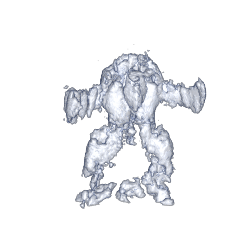
volume_render_scene('../scenes/airsas/arma_20k/reconstructed_scenes/final_upsampled_scene.mat', '../scenes/airsas/arma_20k/reconstructed_scenes', 'ours', 0.2, 1, 0, 230, 0.5)
The backprojected and our rendered image will be scenes/airsas/arma_20k/reconstructed_scenes/bp.png (shown on left) and scenes/airsas/arma_20k/reconstructed_scenes/ours.png (shown on right), repsectively. These are the results
used in Figure 12 of the main text.
Note that reconstruct.sh simply calls the following commands in order.
backproject.sh: reconstructs the scene with backprojection (the traditional reconstruction method we compare against)pulse_deconvolve.sh: deconvolves the sonar waveforms (step 1/2 of our method)neural_backproject.sh: reconstructs the scene using neural backprojection (step 2/2 of our method)python upsample_network.py: queries the trained network at arbitrary spatial resolution to obtain a complex 3D scene for rendering
It is helpful for debugging/developing purposes to call these steps one at a time when running new scenes or adding new features to the code.
The other scenes have identical steps. For example, to reconstruct the bunny, navigate to the ./airsas/bunny_20k and repeat the above.
Note that each scene may use different hyperparameters --- the .sh scripts for each scene are populated with the hyperparameters used for the paper results.
In the paper, we compare our method against a 'Gradient Descent' baseline, which is our method without using a neural network
to predict the scene. If you wish to run this baseline, add the --no_network flag to neural_backproject.sh.
In accordance with funding agency guidelines: request access to the SVSS dataset by first
contacting Albert W. Reed at awreed@asu.edu.
We will walk through an example of reconstructing the cylindrical target. The other SVSS scenes will follow the same steps.
Create a system_data.pik file for the svss cylinder scene:
cd ./scenes/svss/cylinder
chmod +x create_system_data.sh
./create_system_data <path/to/downloaded_data> ./system_data
This will output a system_data.pik file as well as backprojected imagery to a new directory named ./system_data.
Deconvolving the waveforms:
chmod +x pulse_deconvolve.sh
./pulse_deconvolve ./system_data/system_data.pik ./deconvolved_measurements
The first argument is the system_data.pik we generated in the previous step, and ./deconvolved_measurements
is the output directory.
Reconstruct the scene:
chmod +x neural_backproject.sh
./neural_backproject.sh ./system_data/system_data.pik ./deconvolved_measurements ./nbp_output svss_cylinder_exp_1
The following command will generate .mat file of the final scene in the local directory ./reconstructed_scenes.
python ../../../inr_reconstruction/upsample_network_with_input_args.py \
    --system_data ./system_data/system_data.pik \
    --exp_name svss_cylinder_exp_1 \
    --experiment_dir ./ \
    --inr_config ./nbp_config.json \
    --output_scene_file_name final_scene \
    --output_dir_name reconstructed_scenes \
    --model_path ./nbp_output/svss_cylinder_exp_1/models/004000.tar \
    --sf 2 \
    --flip_z \
    --permute_xy
Render the scene with matlab.
volume_render_scene('../scenes/svss/cylinder/reconstructed_scenes/final_scene.mat', '../scenes/svss/cylinder/reconstructed_scenes', 'ours', 0.2, 1, 2, 180, .4)
This is a rendering of the cylindrical target hovering above the seafloor. It appears to be hovering since the sonar only captures returns from the top of the cylinder.
Download the folder containing the transient measurements and system_data.pik file. Note this command will download approx. 100 gb of data. It may be preferrable to download a single scene by directly opening the google drive link below and downloading data for a single scene.
gdown https://drive.google.com/drive/folders/1bWUpcjJhro5m035W98DHDBYv13PGidRF -O ./simulated_data --folder
https://drive.google.com/drive/folders/1bWUpcjJhro5m035W98DHDBYv13PGidRF?usp=share_link
The folder contains data for 6 simulated scenes: bunny, xyz_dragon, lucy, dragon, buddha, and aramdillo, and the
system_data.pik file which defines the scene geometry. Each scene folder contains transients from the
scene using rendered with our ToF renderer. We simulate sonar
measurements by convolving transients with the sonar transmit waveform. Finally, the folder contains a gt_meshes folder used for evaluation.
We provide an example for reconstructing the buddha object in scenes/simulated/buddha.
Install Pytorch3D with the following commands
conda install -c fvcore -c iopath -c conda-forge fvcore iopath
pip install "git+https://github.com/facebookresearch/pytorch3d.git"
Simulate the sonar waveforms from the transients:
cd <project-dir>/scenes/simulated/buddha
chmod +x simulate_waveforms.sh
./simulate_waveforms <path-to-downloaded-simulated-data>/system_data.pik <path-to-downloaded-simulated-data>/buddha/data_full.npy
Deconvolve the simulated waveforms using:
chmod +x pulse_deconvolve.sh
./pulse_deconvolve.sh system_data_20db.pik
Reconstruct the scene with
chmod +x neural_backproject.sh
./neural_backproject.sh
Note that the simulate_waveforms.sh contains other commented parameters that can be modified, and are
currently configured for the paper results.
We provide code for computing metrics of simulated reconstructions in the evaluate folder.
Generate the ground truth point cloud on surface or volume by running
cd <project-dir>/evaluate
chmod +x main_generate_gt_point_cloud.sh
./main_generate_gt_point_cloud <path-to-gt-buddha.obj>
If the process is killed (perhaps because of an out of memory error), try reducing the gt_n_points and gt_n_points_volume arguments of sampled points in the main_generate_gt_point_cloud.sh. Note that this may result
in different quantitative results than the paper.
Reconstruct 3d mesh from learned model and also calculate the 3d space loss from given point cloud.
python main_mesh_recon_and_3d_space_loss.py \
   --output_dir <choose-output-dir> \
   --system_data_path ../scenes/simulated/buddha/system_data_20db.pik \
   --expname sim_buddha_20db_20k_1 \
   --mesh_name budda \
   --comp_albedo_path ../scenes/simulated/buddha/nbp_output/<expname>/numpy/comp_albedo100000.npy \
   --csv_file_name buddha \
   --gt_mesh_dir <path-to-downloaded-gt-mesh-folder> \
   --thresh 0.2
The point cloud is generated in two ways, directly from INR voxels (comp_albedo), or from reconstructed 3D mesh.
We compute the following metrics
- Surface Chamfer Distance : Chamfer distance based on surface point cloud.
- Volume Chamfer Distance : Chamfer distance based on volume point cloud.
- IoU : Intersection over union using between two voxels built from point cloud.
Install a few more packages used for rendering:
pip install PyWavefront
pip install pyrender
pip install pyrr
pip install lpips
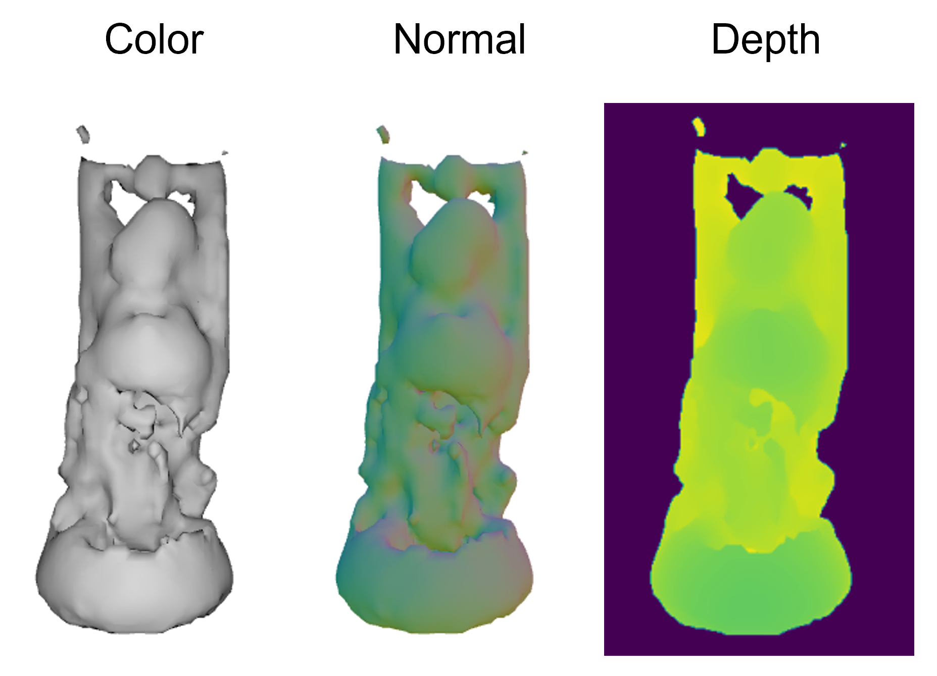
Render the reconstructed mesh's color, normal, and depth at different camera azimuths using:
python main_render.py \
  --n_azimuth 10 \
  --mesh_name budda \
  --expname sim_buddha_20db_20k_1 \
  --render_output_dir ../render_output \
  --gt_mesh_dir <path-to-downloaded-gt-mesh-folder> \
  --recon_mesh_dir <output-dir-from-previous-step> \
  --thresh 0.2 \
  --elevation 0.1 \
  --distance 0.3 \
  --fov 60
- Finally run
main_image_space_loss.shto calculate image space loss (lpips, psnr, mse...) on color image or depth image.
Example configurations are provided in .sh files, but please make sure to set it corresponding to your environment.
Find an example of the rendered mesh of reconstructed buddha using our method in ./evaluate/example_images/buddha_rendered_images_v1.0.png.
We also attach the example of each matric in example_metrics folder.
