This package provides helper function to create models for SNV clustering using empirical bayesian methods with the rjags package.
Use devtools to pull the package from GitHub like so:
install.packages("devtools") # If you do not have it yet
require(devtools)
install_github("PaulPyl/JagsCluster")
A valid JAGS model can be created with the createJagsModel function,
which takes as an input parameter the number of samples (nSamples) and
outputs a text definition of a JAGS model for a series with nSamples
many samples in it.
require(JagsCluster)

## Loading required package: JagsCluster

## Loading required package: rjags

## Loading required package: coda

## Linked to JAGS 4.2.0

## Loaded modules: basemod,bugs

## Loading required package: ggplot2

## Loading required package: reshape2

## Loading required package: cowplot

##
## Attaching package: 'cowplot'

## The following object is masked from 'package:ggplot2':
##
##     ggsave

theModel <- createJagsModel(nSamples = 3)
cat(theModel)

## model {
## # Likelihood:
## for( i in 1 : Nsnvs ) {
##   clust[i] ~ dcat(cluster.weight[1:Nclust])
##   count.1[i] ~ dbin(snv.center.1[i], coverage.1[i])
##   snv.center.1[i] <- cluster.center.1[clust[i]]
##   count.2[i] ~ dbin(snv.center.2[i], coverage.2[i])
##   snv.center.2[i] <- cluster.center.2[clust[i]]
##   count.3[i] ~ dbin(snv.center.3[i], coverage.3[i])
##   snv.center.3[i] <- cluster.center.3[clust[i]]
## }
## # Priors:
## for ( clustIdx in 1 : Nclust ) {
##   cluster.center.1[clustIdx] ~ dunif(0, 1)
##   cluster.center.2[clustIdx] ~ dunif(0, 1)
##   cluster.center.3[clustIdx] ~ dunif(0, 1)
##   delta[clustIdx] ~ dgamma(alpha1, alpha2)
##   cluster.weight[clustIdx] <- delta[clustIdx] / sum(delta[])
## }
## alpha1 ~ dbeta(shape1, shape2)
## alpha2 ~ dbeta(shape1, shape2)
## }
The input data is expected to be a list with two elements named
Support and Coverage, each of those is a matrix with n rows and
m columns where n is the number of SNVs and m is the number of
samples. Usage of meaningful row and column names is encouraged.
We can simulate some data to demonstrate the modelling functionality:
sDat <- simulateData(nSamples = 3, nSNVs = 100, nClusters = 3, meanCoverage = c(60, 120, 180))
lapply(sDat, head)

## $Coverage
##       sample_a sample_b sample_c
## snv_1       59      114      188
## snv_2       61      114      175
## snv_3       44      125      162
## snv_4       47      123      193
## snv_5       62      136      185
## snv_6       48      124      181
##
## $Support
##       sample_a sample_b sample_c
## snv_1       46       64      145
## snv_2       43       55       77
## snv_3       37       42       95
## snv_4       30       64      149
## snv_5       48       57       80
## snv_6       39       55      102
The model is run by a call to the clusterSamples function, giving the
data as input as well as a number of parameters for the clustering
algorith. We will leave them at the default settings for now, eventhough
that will try to fit 10 clusters and we know we simulated only 3.
clusteringResult <- clusterSamples(sDat)

## Compiling model graph
##    Resolving undeclared variables
##    Allocating nodes
## Graph information:
##    Observed stochastic nodes: 300
##    Unobserved stochastic nodes: 142
##    Total graph size: 1119
##
## Initializing model
rjags will produce some output including a progress bar of the modelling process.
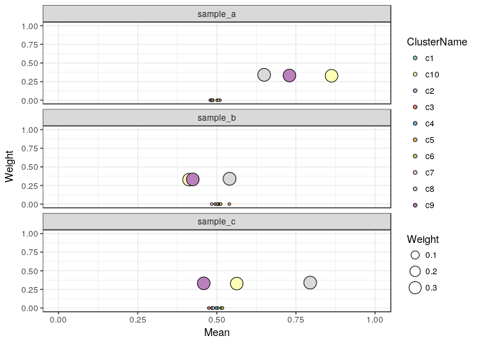
Let's plot the cluster weights and mean allelic frequencies of the result:
plotClusterWeights(clusteringResult) + scale_fill_brewer(palette = "Set3")
In this plot we see three clusters with ~33% Weight (which makes sense since we simulated 3 clusters of equal size), the other clusters have weights close to 0.
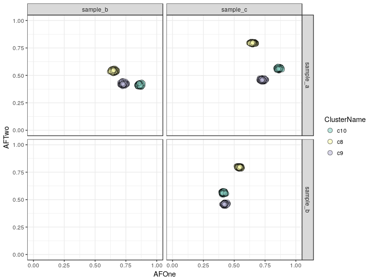
plotClusters(clusteringResult, mode = "point") + scale_fill_brewer(palette = "Set3")
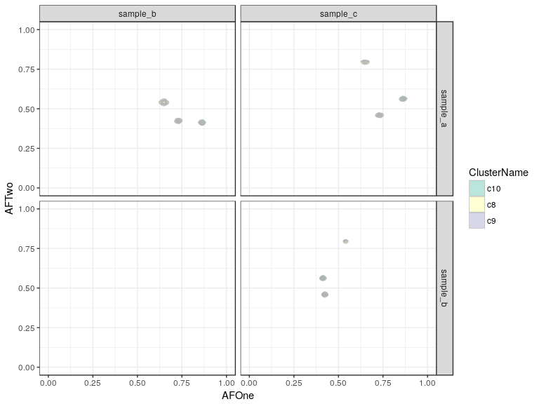
plotClusters(clusteringResult, mode = "density2d") + scale_fill_brewer(palette = "Set3")
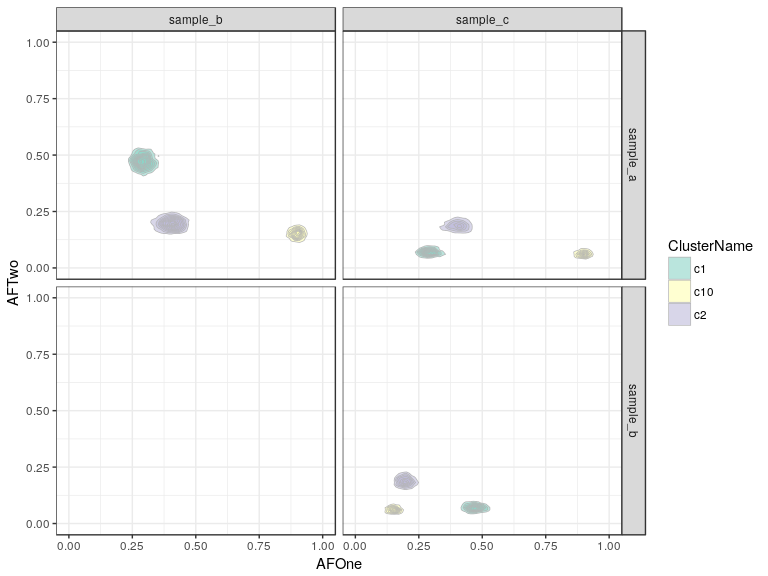
The density version of this plot is not very helpful in this case of simulated data, which are not very noisy at all, this can be more informative if your clusters show a wide spread or strangely shaped clouds, to determine the underlying density. If the coverage is lower the data becomes more noisy and if the number of SNVs is lower the clusters will also be less well-defined, an example is shown below:
sDatNoisy <- simulateData(nSamples = 3, nSNVs = 40, nClusters = 3, meanCoverage = c(20, 30, 40))
clusteringResultNoisy <- clusterSamples(sDatNoisy)

## Compiling model graph
##    Resolving undeclared variables
##    Allocating nodes
## Graph information:
##    Observed stochastic nodes: 120
##    Unobserved stochastic nodes: 82
##    Total graph size: 519
##
## Initializing model

cp <- plotClusters(clusteringResultNoisy, mode = "density2d") + scale_fill_brewer(palette = "Set3")
cp
Another way to look at this is to plot the SNVs annotated with the clusters they were assigned to:
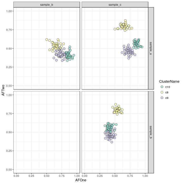
sp <- plotResultSNVs(clusteringResult, mode = "point") + scale_fill_brewer(palette = "Set3")
sp
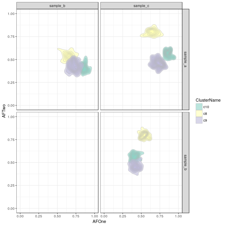
It can be useful to look at this as a density plot, in case too many points overlap and it is not easy to make out the shape and local density of the clusters.
sp <- plotResultSNVs(clusteringResult, mode = "density2d") + scale_fill_brewer(palette = "Set3")
sp
Here we see our three clusters of simulated SNVs and their respective allelic frequencies in the three samples.
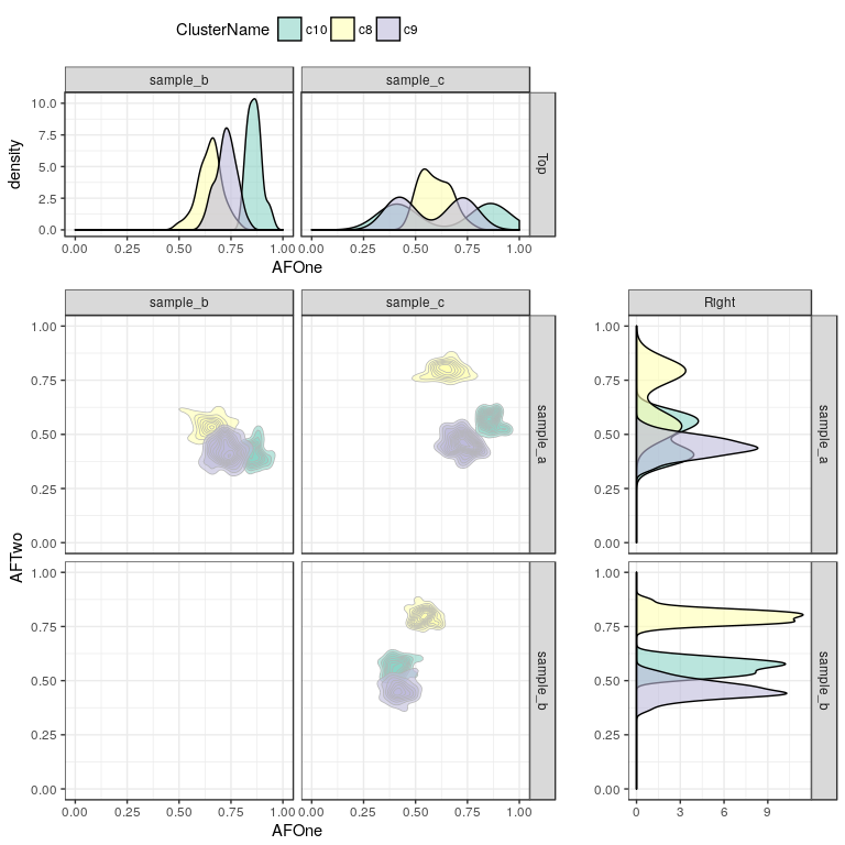
Sometimes it can be interesting to add marginal distribution densities to those plots as well:
addMarginals(sp, scale_fill_brewer(palette = "Set3"))

## Scale for 'fill' is already present. Adding another scale for 'fill',
## which will replace the existing scale.
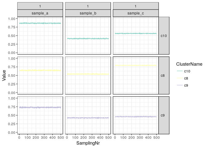
A more in-depth look can be had by tracing the actual allele frequencies of the clusters as they were sampled from the mixture model. Here we plot only clusters which contain at least 1% of SNVs in the final estimate.
plotChains(clusteringResult, minWeight = 0.01) + ylim(0,1) + scale_colour_brewer(palette = "Set3")
We see that the model has converged very well and in all samples the clusters are very stable in their respective estimated alelle frequencies. Since this is simulated data we did expect such behaviour and in real-world examples the clusterin can be much more unstable. Typically it is advisable to filter the input data strictly and try to focus on SNVs where there is a lot of evidence, i.e. where the coverage is high, so that the estimated AFs can be very precise.
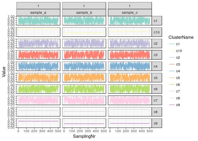
If we allow for all clusters to be plotted we see that the clusters with
low weight do not converge at all and are all over the place, this is
not a problem however, since when the clusters contain no data the prior
probability is never updated and so they sample from a uniform
distribution between 0 and 1, which is expected.
plotChains(clusteringResult, minWeight = 0) + ylim(0,1) + scale_colour_brewer(palette = "Set3")
