This is a Python 3 implementation of Stokesian Dynamics for spherical particles of different sizes.
- 0. Contact details and how to contribute
- 1. What is Stokesian Dynamics?
- 2. What can this software do?
- 3. What are its limitations?
- 4. System requirements
- 5. How to set up the software
- 6. What's in each folder?
- 7. How to test that the software is working
- 8. How to run your first simulation
- 9. Reading and plotting the output
- 10. Changing the inputs
- 11. Examples and comparisons with the literature
- 12. Increasing the number of particle size ratios available
- 13. Known issues
- This code is written by Adam Townsend (adamtownsend.com, @Pecnut).
- Feel free to post in the discussion forum with questions or ideas if you are happy to comment publicly.
- You can also create a new issue in the GitHub repository if you want to report a bug.
Stokesian Dynamics is a microhydrodynamic, low Reynolds number approach to modelling the movement of suspensions of particles in fluids which considers the interaction of particles with each other against a Newtonian background solvent. The fluid is modelled using the Stokes equations. It is typically chosen for its suitability for three-dimensional simulation with low calculation and time penalty.
In the most basic case, Stokes’ law states that a single sphere of radius a, travelling with a velocity U in an unbounded Newtonian fluid of viscosity μ, in a low Reynolds number regime, experiences a drag force, F, of F = −6πμaU.
Stokesian Dynamics, at its heart, is an extension of this linear relationship between the force acting on a particle and the velocity at which it travels. As a method, it is adaptable and continues to be used in the field, providing some interesting insight into the behaviour of particle suspensions. Validations with experiments have shown it to provide results within acceptable error.
The Stokesian Dynamics recipe can be summarised as follows:
- Compute long-range interactions between particles. This is done by using a truncated expansion of the boundary integral equation for unbounded Stokes flow. For periodic domains, this is done by using the Ewald summation method.
- Compute short-range lubrication between particles. This is done by interpolating pre-computed results on a pairwise basis.
- Combining the two.
It is fully explained (in painful detail) in my PhD thesis.
This software allows you to place spherical particles in a fluid, apply some forces to them, and see how they move. You can also move the fluid in some way and see how the particles react to that. You can have a play with a simpler implementation of Stokesian Dynamics in this nice online version.
In particular, this software has the following features:
- Fully 3D simulation
- Free choice of number of particles
- Choice of simulating particles in an unbounded fluid ('non-periodic') or in a periodic domain
- Free choice of spherical particles sizes (up to n different sizes for low n)
- Choice to include bead-and-spring dumbbells, formed of pairs of (usually smaller) spherical particles, as a way to introduce viscoelasticity into the background fluid
- Free choice of particle interaction forces
- Choice of whether to include long-range hydrodynamic forces or not (M∞)
- Choice of whether to include lubrication forces or not (R2B,exact)
- Choice of Euler, two-step Adams–Bashforth or RK4 timestepping
- Choice of how often to find (M∞)⁻¹, a matrix which varies slowly and takes a long time to compute, hence is typically computed every 10 timesteps.
- For each spherical, non-bead-and-spring particle in the system, the software takes the forces and torques you want to apply to it, as well as the background fluid shear rate (F, T and E), and gives you the particle velocities, angular velocities and stresslets (U, Ω and S). It can also do FTS to UΩE, for when you want to specify stresslets instead of the background shear rate; and U₁F₂TE to F₁U₂ΩS, for when there are some particles whose velocities you want to fix while letting some other particles move under specified forces (e.g. when you want to fix some particles as walls). See the settings documentation for more information.
- Time-to-completion estimates
- Emails you on completion
- Output stored in convenient .npz format
- Video generation scripts to watch the particle behaviour
Speed and memory are the greatest limitations of the software. Loosely speaking, for a concentrated system of s spheres and d dumbbells, the memory, in bytes, required, is 48(11s + 6d)².
This is an implementation in Python, using Numba for speed. It has been tested with Python 3.9 and requires the following Python packages:
- matplotlib, numba, numpy, psutil, pytest, scipy
Section 5 below explains how to install these packages.
The software does not need to be installed. It can be run directly from the folder it is downloaded into.
- Download the software into its own folder. The easiest way to do this is to navigate to the folder in Terminal that you want to download the Stokesian Dynamics folder into, and to type
git clonefollowed by the address you find at the top of this page when you change the SSH dropdown to HTTPS (the address you need should look something likehttps://github.com/Pecnut/stokesian-dynamics.git). - Install the required Python packages, or confirm that they are already installed (see section 4), by typing
pip install -r requirements.txtin Terminal. - You can speed up the code using Numba. Numba is a Python package which can dramatically speed up functions. It does this by optimising functions which are 'decorated' with the
@njitlabel in the code. A number of core functions in this software are decorated with this label. Numba is turned OFF by default; turn it on by changingconfig.DISABLE_JITin settings.py toFalse. The optimisation happens the first time a function is called, so when Numba is enabled, the first timestep will be slow, but the rest will be very fast. It is therefore worth turning on for most simulations.
The software should now be ready to run.
The main folder contains a number of subfolders. They are:
stokesian_dynamics: The main Stokesian Dynamics software is in this folder and you should navigate to this folder in Terminal to run the software.find_resistance_scalars: This contains code to calculate the resistance scalars for particles of different sizes, if you would like to increase the number of particle size ratios available, and contains the scripts referred to in Townsend, 2023. See section 12.docs: This contains documentation for the software which is additional to this README file.examples: This contains example Python scripts which show how to analyse the results of the software for some example cases. See section 11.tests: This contains tests for the software, which you can run to check that the software is working. See section 7.
The software comes with a number of tests which compare the output of the simulation to pre-computed analytic results for two-particle systems in a non-periodic domain. These are stored in the tests folder, but you don't need to visit this folder in order to run them. Instead:
- Follow the steps in section 5
- Navigate to the main folder in Terminal and type
python -m pytest.
This will run all the tests in the tests folder. A successful run will output something like:
============================= test session starts ==============================
platform darwin -- Python 3.9.13, pytest-7.1.2, pluggy-1.0.0
rootdir: /.../stokesian-dynamics
plugins: anyio-3.5.0
collected 1 item

tests/test_all.py .                                                      [100%]

============================== 1 passed in 4.34s ===============================
- Follow the steps in section 5.
- Navigate to the
stokesian_dynamicsfolder inside the main folder in Terminal. - Type
python run_simulation.py 2 1 0.5 1.
This will run a simulation of particles, starting at the positions defined in position setup number 2, under the forces defined in input setup number 1, with timestep 0.5, and for 1 frame.
This simulation is of three spheres of radius 1, arranged horizontally at x = –5, 0 and 7. They are all given a downwards force of F = 1. The domain is an infinite fluid (i.e. non-periodic).
A successful run will output something like:
+--------------------+-------------------+-----------------------+--------------------+
| Setup:    2        | Minfinity: ON     | Matrix form: FTE                           |
| Input:    1        | R2Bexact:  ON     | Solve using: Fast R\F | Video:    OFF      |
| Frames:   1        | Bead-bead: ON     | Inv M every: 10       | Memory:  ~51 KB    |
| Timestep: 0.5      | Timestep:  Euler  | Periodic:    OFF      |                    |
+--------------------+-------------------+--------------------------------------------+
| Save every: 1      | Save after: 0     | Machine: ComputerName                      |
+--------------------+-------------------+--------------------------------------------+
[Generating 1901111302-s2-i1-1fr-t0p5-M10-gravity]
                        [ Minfy  ] [invMinfy] [R2Bex'd'] [ U=R\F  ] [ Saving ] [MaxMemry] [[ Total  ]] [TimeLeft] [ ETA ]
Processing frame 1/1... [    0.0s] [    0.0s] [    0.0s] [    0.1s] [    0.0s] [ 35.8 MB] [[    0.1s]] [    0.0s] [13:02]
[Total time to run     0.6s]
[Complete: 1901111302-s2-i1-1fr-t0p1-M10-gravity]
The top box gives a summary of the job that is executing, including an estimate of how much memory will be required.
After each frame is generated, a list of timings is shown for each part of the process (respectively, creating M∞, inverting it, creating R2B,exact, solving the mobility formulation, saving the data to disk). Then the maximum memory used in this step is shown. Finally, a countdown to completion and an estimated time of completion is shown.
You can find the outputs of all your simulations in the output folder inside stokesian_dynamics. Output files are named yymmddhhmm-s407-i700-1fr-t0p005-...npz, where yymmddhhmm is replaced by the simulation timestamp in that format (so 2412251500 for 3pm on Christmas Day 2024).
The output is in the convenient .npz format, a zipped Numpy file. It contains various useful Numpy arrays. It can be read with the following Python code, where you have to substitute the filename for FILENAME:
import numpy as np
data = np.load("output/FILENAME.npz")
particle_centres = data['centres']
dumbbell_displacements = data['deltax']
forces_on_particles = data['Fa']
forces_on_dumbbells = data['Fb']
internal_forces_on_dumbbells = data['DFb']
particle_stresslets = data['Sa']
particle_rotations = data['sphere_rotations']
The file plotting/plot_positions.py plots the particle positions from a saved file at a given frame number.
Set filename and frameno to be the name of the output file and the frame number you want to plot. You can also set viewing_angle and viewbox_bottomleft_topright to change the viewing angle and the size of the view box.
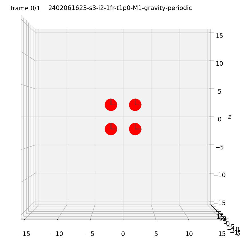
For example, here I have run python run_simulation.py 3 2 1 1 fte on 6 February 2024 at 16:23. It has created a file called 2402061623-s3-i2-1fr-t1p0-M1-gravity-periodic.npz in the output folder. Changing filename in plot_positions.py to 2402061623-s3-i2-1fr-t1p0-M1-gravity-periodic and then running the script plots the positions of the particles at the (by default) first frame of this simulation.
The file plotting/make_video.py creates a video of the particle positions from a saved file and places it in the output_videos folder.
By default, it creates a video of the entirity of the most recent simulation. You can override the filename and the number of frames to include in the video by changing the variables filename, num_frames_override_start and num_frames_override_end at the top of the file. You can also set viewing_angle and viewbox_bottomleft_topright to change the viewing angle and the size of the view box.
All files which contain the inputs for the Stokesian Dynamics simulation are contained in the stokesian_dynamics folder.
All possible input choices are contained in settings.py and are documented in the settings documentation.
The most important four, setup_number, input_number, timestep, num_frames are set at the top but can also be overwritten by explicitly stating them at the command line, as we did in section 8 above (python run_simulation.py 2 1 0.5 100). Simply running python run_simulation.py will use the values stated in settings.py.
-
The variable
setup_numbercorresponds to the initial particle configuration in setups/positions.py, containing initial particle positions and sizes in a big 'if' list. -
The variable
input_numbercorresponds to the forces, torques and background fluid velocities (as well as anything else being imposed on the particles) in setups/inputs.py.
When creating new setup_number and input_number cases, use the existing cases as templates.
See the settings documentation for more information.
Note: as received, the software is only able to perform simulations with particles of size ratio 1:1, 1:10 and 1:100. To increase this, see section 12.
The most common use case is that you want to impose particle forces (F), particle torques (T) and background strain rate (E), and therefore that you want to output particle velocities (U), particle angular velocities (Ω) and particle stresslets (S). However, this is not the only option in this code. You may want to impose F, T, S and output U, Ω, E. Or you may wish to impose a mix of particle velocities and forces, for example if you have some particles acting as rigid bodies or lids, and some particles being free to move. So long as all particles in the system have some behaviour imposed on them, you can implement this behaviour in the code by changing the variable input_form in settings.py, or by adding an appropriate flag to the end of the command line:
- Impose FTE: use
fteor nothing - Impose FTS or you are just running a simulation with no spheres, only dumbbells: use
fts - Impose some U, some F, and TE: use
ufte.
Examples:
- Usual FTE behaviour:
python run_simulation.py 2 1 0.5 100orpython run_simulation.py 2 1 0.5 100 fte - Mix of U/F, along with TE:
python run_simulation.py 6 5 1 1 ufte
If you see errors involving 'pippa', it's normally because you have got this wrong.
Within the stokesian_dynamics folder, the files setups/positions.py and setups/inputs.py come with some example setups for Stokesian Dynamics simulations. In these examples, the downward vertical direction is the –z direction. Set view_graphics = True in settings.py to watch these simulations.
Durlofsky, Brady & Bossis, 1987. Dynamic simulation of hydrodynamically interacting particles. Journal of Fluid Mechanics 180, 21–49. Figure 5.
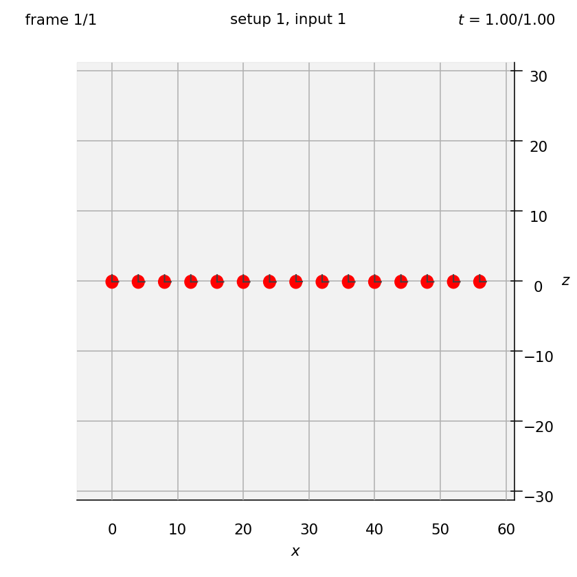
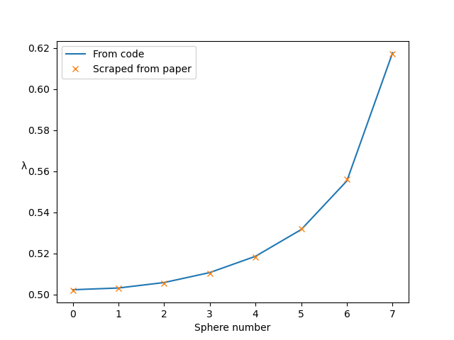
This test case looks at horizontal chains of 5, 9 and 15 spheres sedimenting vertically. The instantaneous drag coefficient, λ=F/(6πμaU), is measured for each sphere in the chain, in each case. Here we set up the chain of length 15. We can reproduce the figure in the paper by running this simulation for 1 timestep with Euler timestepping (set timestepping_scheme = 'euler' in settings.py). We just need to read the velocity U of each sphere and calculate λ.
Set view_graphics = True and viewbox_bottomleft_topright = np.array([[-4, 0, -30], [60, 1, 30]]) in settings.py to see the whole chain. As we will run for only 1 timestep, the chain will not move far from its initial position.
Run python run_simulation.py 1 1 1 1 fte (position setup number 1, forces input 1, with a timestep of 1 [arbitrary choice] for 1 timestep, specifying forces, torques and rate of strain).
Follow the instructions in examples/example-a.py to produce the following graph, comparing the results from this simulation to the figure in the paper:
Durlofsky, Brady & Bossis, 1987. Dynamic simulation of hydrodynamically interacting particles. Journal of Fluid Mechanics 180, 21–49. Figure 5.
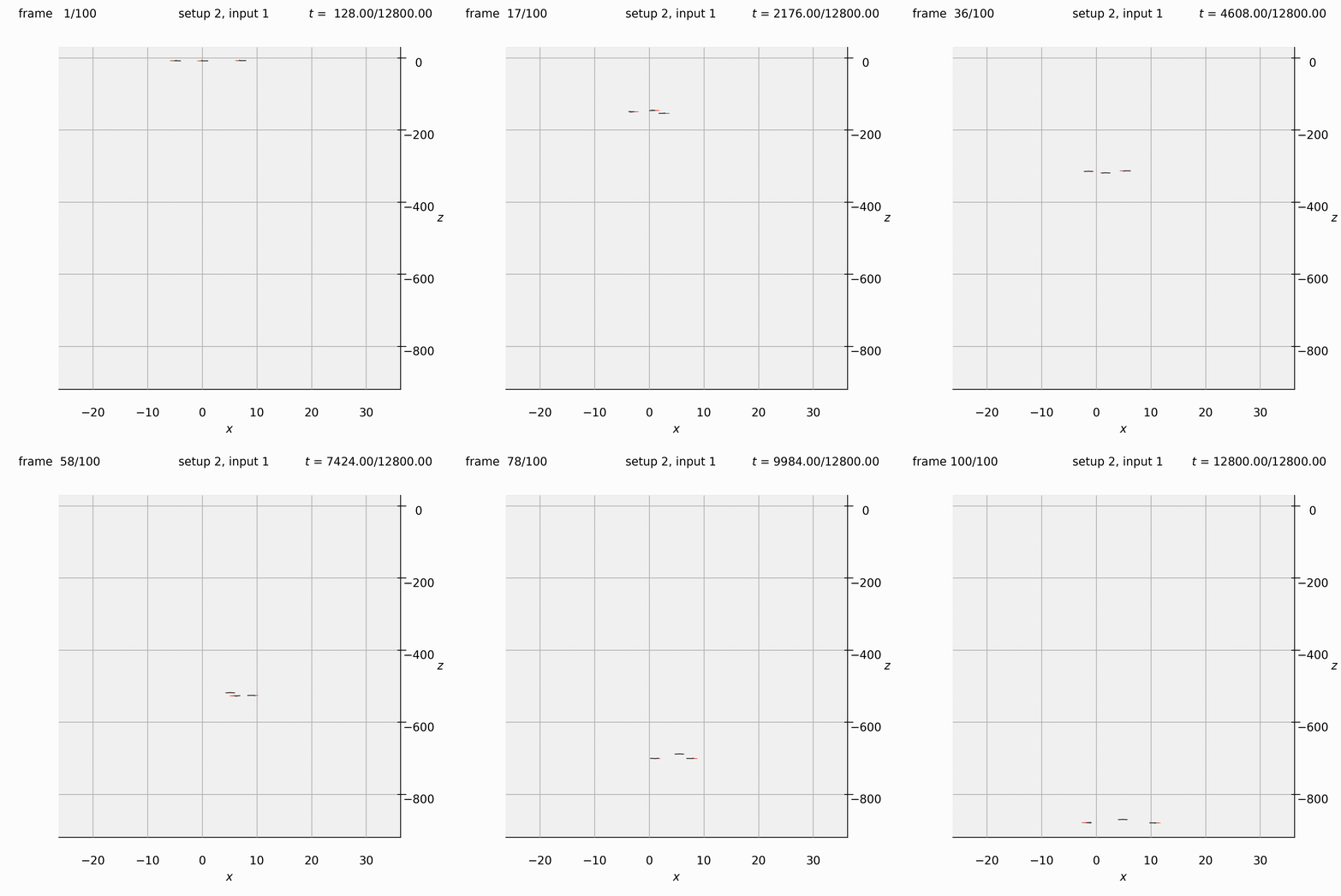
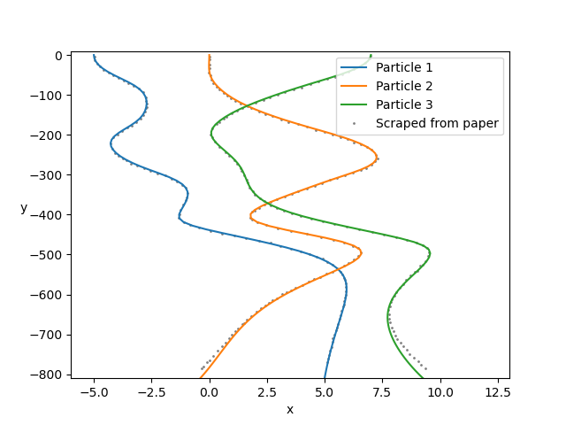
This test case considers three horizontally-aligned particles sedimenting vertically, and looks at their interesting paths over a large number of timesteps. Use RK4 timestepping (set timestepping_scheme = 'rk4') and ensure invert_m_every is set to 1, in order to recover the same particle paths.
Set view_graphics = True and viewbox_bottomleft_topright = np.array([[-25, 0, -900], [35, 1, 10]]) in settings.py to watch the spheres fall. As this view box is not square, the spheres will appear to be squashed.
Run python run_simulation.py 2 1 128 100 fte.
Follow the instructions in examples/example-b.py to produce the following graph, comparing the results from this simulation to the figure in the paper:
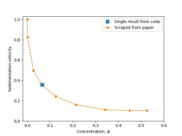
Sierou & Brady, 2001. Accelerated Stokesian Dynamics simulations. Journal of Fluid Mechanics, 448, 115--146. Figure 9. Correction to Brady, Phillips, Lester & Bossis, 1988. Dynamic simulation of hydrodynamically interacting suspensions. Journal of Fluid Mechanics 195, 257–280. Figure 1.
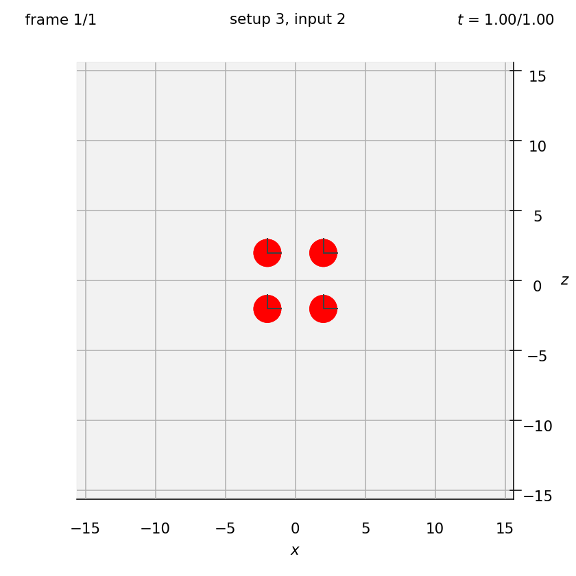
A simple cubic array sediments vertically under a constant force. The velocity is measured for different particle concentrations. Vary the concentration by altering the cubic lattice size.
Note that a periodic domain is activated by setting box_bottom_left and box_top_right to be different in setups/settings.py. Make sure how_far_to_reproduce_gridpoints ≥ 2 for accurate results.
Set view_graphics = True and viewbox_bottomleft_topright = np.array([[-15, 0, -15], [15, 1, 15]]) (the default) in settings.py to see the unrepeated cubic array in the xz-plane. As we will run for only 1 timestep, the array will not move far from its initial position.
Run python run_simulation.py 3 2 1 1 fte.
Follow the instructions in examples/example-c.py to produce the following graph, comparing the results from this simulation to the figure in the paper:
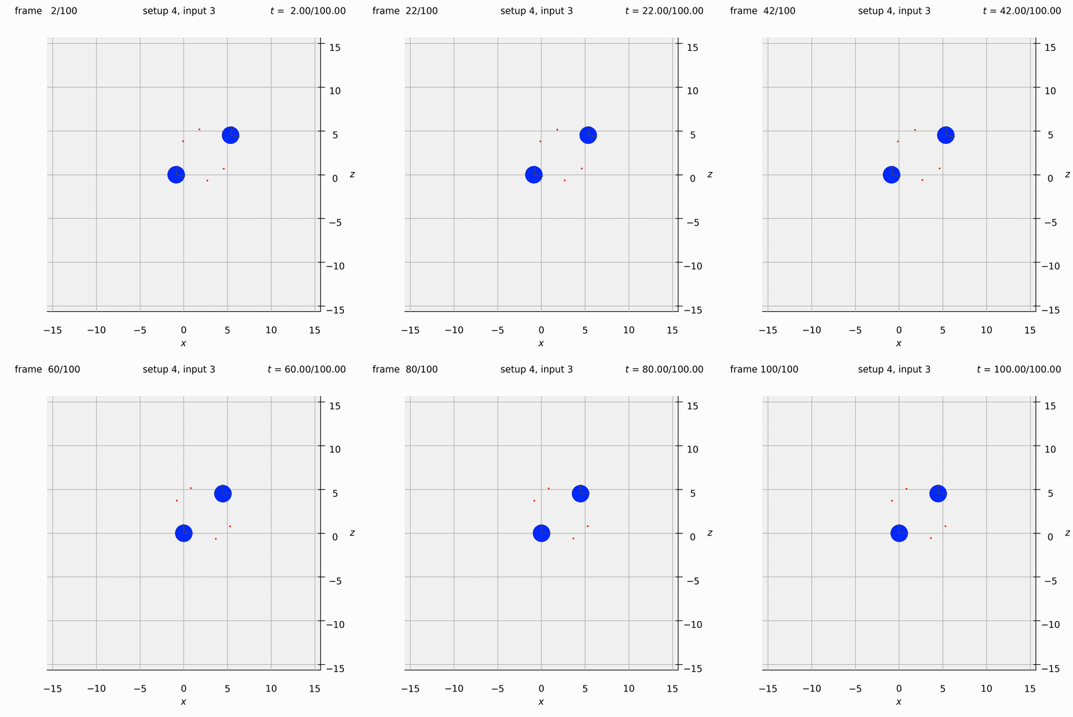
Arrange two large spheres and two dumbbells in a square, then put in an oscillatory background flow. Set the dumbbell spring constant.
Set view_graphics = True and viewbox_bottomleft_topright = np.array([[-15, 0, -15], [15, 1, 15]]) (the default) in settings.py to see the motion of the particles in the xz-plane.
Run python run_simulation.py 4 3 1 100 fte.
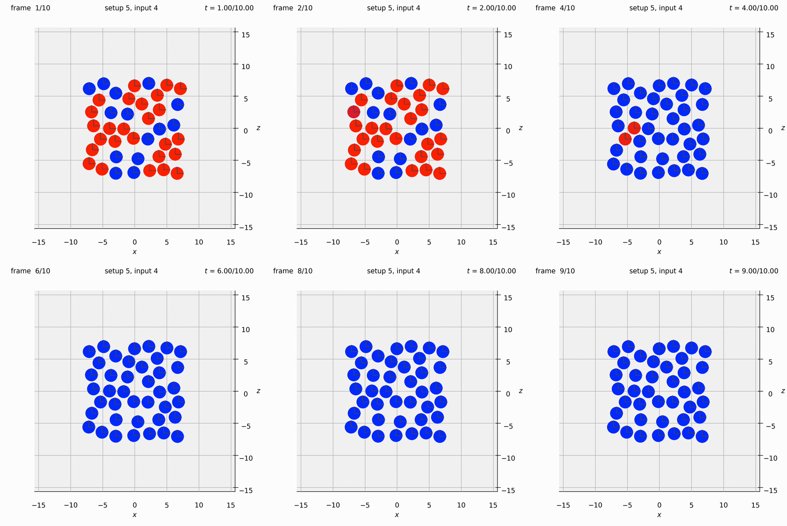
Randomly arrange spheres in a 2D box in the xz-plane. Place a repulsive force between them so that they spread out.
Set view_graphics = True and viewbox_bottomleft_topright = np.array([[-15, 0, -15], [15, 1, 15]]) (the default) in settings.py to see the motion of the particles in the xz-plane. The spheres change colour from red to blue as the total force acting on them reduces.
Run python run_simulation.py 5 4 1 10 fte.
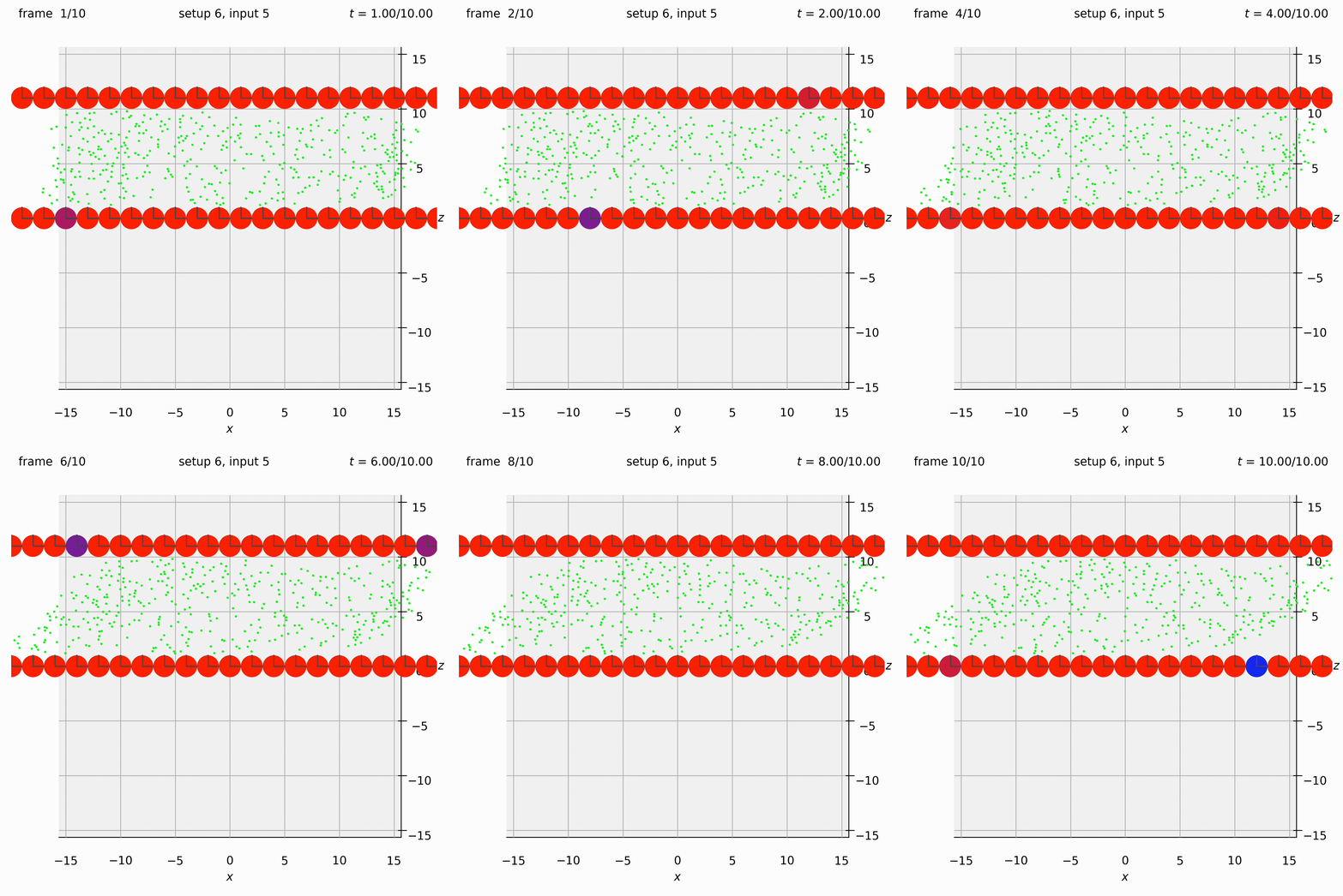
Create two walls of spheres, with dumbbells randomly arranged between them. Specify the velocity of the walls. Observe what happens to the dumbbells.
This time we need the ufte flag because we are specifying velocities.
Set view_graphics = True and viewbox_bottomleft_topright = np.array([[-15, 0, -15], [15, 1, 15]]) (the default) in settings.py to see the motion of the particles in the xz-plane.
Run python run_simulation.py 6 5 1 10 ufte.
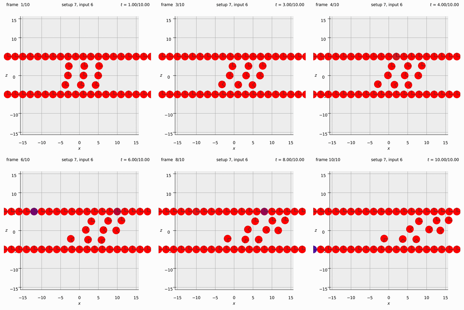
Create two walls of spheres, with a 3×3 array of spheres between them. Specify the velocity of the walls, but also give the spheres in the middle a force to the right.
We need the ufte flag because we are specifying velocities.
Set view_graphics = True and viewbox_bottomleft_topright = np.array([[-15, 0, -15], [15, 1, 15]]) (the default) in settings.py to see the motion of the particles in the xz-plane.
Run python run_simulation.py 7 6 1 10 ufte.
When specifying forces for some spheres and velocities for other spheres, be careful that every sphere is given either a force or a velocity.
Use the function same_setup_as('FILENAME', frameno=0) in setups/positions.py to copy the setup from a certain file, starting at a given frame number.
Run python run_simulation.py 8 1 1 1 fte.
By default, the software comes with the precomputed resistance data for particles of size ratio 1:1, 1:10 and 1:100. To increase this:
- Open the folder find_resistance_scalars
- Add the size ratios to the file values_of_lambda.txt
- Then follow the instructions in section 3 of find_resistance_scalars/README.md
This last step requires you to compile some Fortran code and run a Python script; the instructions are all in the aforementioned README file. Calculating this data can take about an hour on a contemporary laptop, so give yourself some time.
The method is from:
- Townsend, 2023. Generating, from scratch, the near-field asymptotic forms of scalar resistance functions for two unequal rigid spheres in low Reynolds number flow, Physics of Fluids 35(12), 127126.
- Wilson, 2013. Stokes flow past three spheres, Journal of Computational Physics 245, 302–316.
This error occurs when you try to plot an image on a remote server without a working display.
Remedy: Set view_graphics = False in settings.py.
Reason: If view_graphics = True, the timesteps are looped over using animation.FuncAnimation, which allows you to see what's going on in the simulation in 'real time'. If view_graphics = False, then the timesteps are looped over just with a for loop, bypassing the plotting functionality completely.
This is a common error when working on a remote server. If you set view_graphics = False, you can pick up the output data from the /output/ folder and create the video yourself on your own machine.
This error occurs when the main body of the code (generate_frame) has not been called before the code tries to finish.
Probable remedy: Set view_graphics = False in settings.py or, remove matplotlib.use('agg') if you have added this.
Reason: If view_graphics = True, the timesteps are looped over using animation.FuncAnimation, which allows you to see what's going on in the simulation in 'real time'. If view_graphics = False, then the timesteps are looped over just with a for loop, bypassing the plotting functionality completely.
The normal cause of this error is that view_graphics = True, but despite this, animation.FuncAnimation has not functioned correctly. This happens if you change the matplotlib backend to a backend such as Agg which does not require a working display: see the Agg backend is not compatible with animation.FuncAnimation.
