The goals / steps of this project are the following:
- Compute the camera calibration matrix and distortion coefficients given a set of chessboard images.
- Apply a distortion correction to raw images.
- Use color transforms, gradients, etc., to create a thresholded binary image.
- Apply a perspective transform to rectify binary image ("birds-eye view").
- Detect lane pixels and fit to find the lane boundary.
- Determine the curvature of the lane and vehicle position with respect to center.
- Warp the detected lane boundaries back onto the original image.
- Output visual display of the lane boundaries and numerical estimation of lane curvature and vehicle position.
Rubric Points
Here I will consider the rubric points individually and describe how I addressed each point in my implementation.
You're reading it!
The code for this step is contained in the second code cell of the IPython notebook located in "./code.ipynb".
I start by preparing "object points", which will be the (x, y, z) coordinates of the chessboard corners in the world. Here I am assuming the chessboard is fixed on the (x, y) plane at z=0, such that the object points are the same for each calibration image. Thus, objp is just a replicated array of coordinates, and objpoints will be appended with a copy of it every time I successfully detect all chessboard corners in a test image. imgpoints will be appended with the (x, y) pixel position of each of the corners in the image plane with each successful chessboard detection.
I then used the output objpoints and imgpoints to compute the camera calibration and distortion coefficients using the cv2.calibrateCamera() function. I applied this distortion correction to the test image using the cv2.undistort() function and obtained this result:
See above.
2. Describe how (and identify where in your code) you used color transforms, gradients or other methods to create a thresholded binary image. Provide an example of a binary image result.
First, the input image is converted from BGR to greyscale. Then I use a combination of Sobel thresholding on both the x and y direction. I found that a kernel size of 7 and threshold range of 20-100 for both directions gives the best result when the two output images are ANDed together. (Code is in cell 3)
Next, gradient magnitude and gradient direction are applied to the greyscale input image, resulting in the images shown below. These two images are also ANDed together.
The final thresholding technique applied is colour thresholding on the S channel of a HLS converted image.
The three outputs are then overlayed (ORed) into a single image, as seen below.
The code to produce the final binary image can be viewed in the Pipeline function in cell 5
3. Describe how (and identify where in your code) you performed a perspective transform and provide an example of a transformed image.
The code for my perspective transform can be found in the bottom of cell 2. I captured a frame from the video showing a straight section of road and then used an image editing program to find the coordinates of a rectangular section suitable for perspective transformation. This section contains exactly three center lines, so it can also be used to estimate the scale of the photo. The destination points were simply the width and height of the image, with a 300 pixel offset along the sides to allow for any curvature.
offset = 300
src = np.float32([(331, 648), (589, 455), (696, 455), (1021, 648)])
dst = np.float32([(offset, img_size[1]), (offset, 0), (img_size[0]-offset, 0),  (img_size[0]-offset, img_size[1])])
4. Describe how (and identify where in your code) you identified lane-line pixels and fit their positions with a polynomial?
First, I OR thgether the current and previous binary image to help fill in the gaps that sometimes appear. Then I use a sliding window (In code cell 4) to estimate the position of the lane lines.
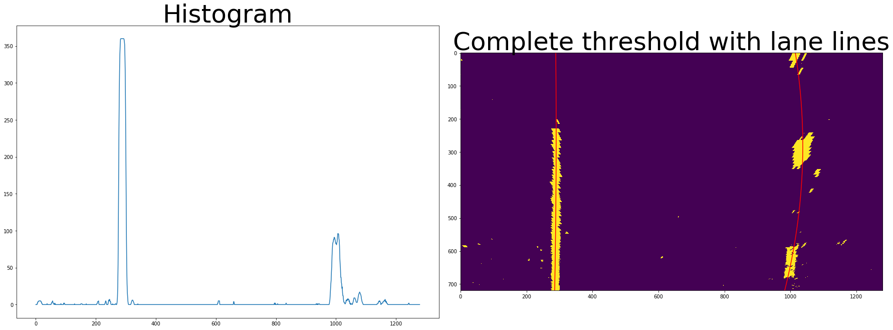
This works by taking a Histogram of the binary image, and finding the two higest peaks. These are our starting points for the lane lines at the bottom of the image.
Then the image is sectioned into 9 horizontal slices. A sliding window is "slid" across each half of the slice, and the area containing the most illuminated pixels is assumed to be the location of the lane line. This is repeated left and right for all 9 slices.
The cordinates from the sliding window result is fed into the np.polyfit function, which uses the "least squares" technique to fit a 2nd order polynomial. This polynomial is redwawn on the image below for example only, in the video a green polygon is overlayed on the output image.
The image below shows one of the hardest images for detection, where you can see that the right hand lane is slightly incorrect, despite the line being correctly drawn through the center of the lane markings. (Perhaps the lane markings are wrong?) To help overcome this I run the polynomial coefficients through a low pass filter. This limits the rate of change to 15% per frame, so if there is a tempory glitch as there is in this spot, a single bad frame or two won't adversly affect detection. (It was turned off to produce this image)
5. Describe how (and identify where in your code) you calculated the radius of curvature of the lane and the position of the vehicle with respect to center.
I did this in the bottom of cell 4. First, the lane line coordinates are scaled into world space (from pixels to metres), and then a new polynomial is created. I did try scaling the polynomial coefficients directly, but ran out of time to get it working. The radius of curvature can then be calculated using the scaled polynomial coefficients.
The lane deviation is calculated by finding the midpoint of the two lanes, and then subtracting this from the midpoint of the image (which is assuming the camera view is positioned in the center of the car).
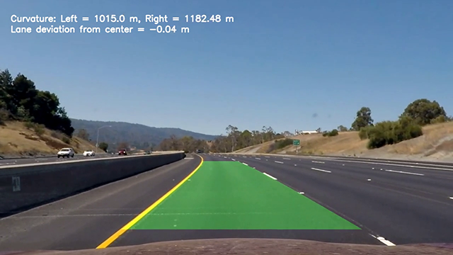
The results from both measurements are written onto the final output image.
6. Provide an example image of your result plotted back down onto the road such that the lane area is identified clearly.
I implemented this step in the Pipeline function in cell 5. Here is an example from a frame of the video.
1. Provide a link to your final video output. Your pipeline should perform reasonably well on the entire project video (wobbly lines are ok but no catastrophic failures that would cause the car to drive off the road!).
Here's a link to my video result
1. Briefly discuss any problems / issues you faced in your implementation of this project. Where will your pipeline likely fail? What could you do to make it more robust?
As previously discussed, I had some trouble with low contrast surfaces like the concrete bridge. As I have completly run out of time I couldn't try anything fancy like calculating a confidence level for the lane detection, and then ignoring any information below a specific confidence threshold. Instead, I just heavily filtered the output to try and minimise noise and unwanted errors.
I also didn't get time to implement faster lane search detection for when the approximate location of the lane lines are known, so a sliding window is used on every frame.


