RNiftyReg: Nifty Registration in R

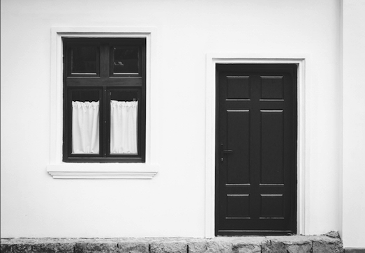
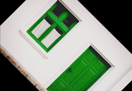
The RNiftyReg package is an R-native interface to the NiftyReg image registration library developed within the Translational Imaging Group at University College London. The package incorporates the library, so it does not need to be installed separately, and it replaces the NiftyReg command-line front-end with a direct, in-memory bridge to R, based on Rcpp.

This README file primarily covers version 2.0.0 of the package and later. The interface was substantially reworked in that version to make it more natural and less verbose, and earlier versions are incompatible. Information on moving from prior versions of RNiftyReg to 2.x is included at the end of this file.

The package can be installed from CRAN, or the latest development version obtained directly from GitHub:

## install.packages("remotes")
remotes::install_github("jonclayden/RNiftyReg")

The mmand package for image processing may also be useful, and is used in some of the examples below.

Reading and writing images
Image registration
Applying and manipulating transformations
Convenience functions
Upgrading to RNiftyReg 2.x

Reading and writing images

RNiftyReg may be used to register and manipulate two and three dimensional images of any sort, although its origins are in medical imaging. Medical images in the standard NIfTI-1 format may be read into R using the readNifti function, which is based on the first-party RNifti package.

library(RNiftyReg)
image <- readNifti(system.file("extdata", "epi_t2.nii.gz", package="RNiftyReg"))

This image is an R array with some additional attributes containing information such as its dimensions and the size of its pixels (or voxels, in this case, since it is a 3D image).

As mentioned above, however, images do not have to be in NIfTI-1 format. Any numeric matrix or array can be used, and standard image formats such as JPEG and PNG can be read in using additional packages. For example,

## install.packages("jpeg")
library(jpeg)
image <- readJPEG(system.file("extdata", "house_colour_large.jpg", package="RNiftyReg"))

Complementary writeNifti and writeJPEG functions are provided by the RNifti and jpeg packages, respectively.

Image registration

Once two or more images have been read into R, they can be registered. Registration is the dual operation of searching a space of transformations for the best way to align two images, and then resampling one image onto the grid of the other. The images need not be the same size or in the same orientation.

There are two main classes of transformation available: linear and nonlinear. Linear, and specifically affine, transforms can represent translation, scaling and rotation in 2D or 3D space. They have up to 12 degrees of freedom and are appropriate to capture global shifts between images. Nonlinear transformations have many more degrees of freedom, and can capture localised distortions between images, but they are more time-consuming to estimate and more complex to work with.

Some sample 3D medical images are included with the package. We begin by registering two brain scan images, of the same person, with different contrasts. First we read them in, and then we pass them to the package's core registration function, niftyreg.

source <- readNifti(system.file("extdata", "epi_t2.nii.gz", package="RNiftyReg"))
target <- readNifti(system.file("extdata", "flash_t1.nii.gz", package="RNiftyReg"))

result <- niftyreg(source, target)

The last command will take a few seconds to complete. The result is a list with a number of components, the most important of which is the resampled source image in target space, result$image.

By default the transformation will be an affine matrix. If we want to allow for a nonlinear transformation, with scope for local deformations between one space and the other, we can perform an additional registration as follows.

result <- niftyreg(source, target, scope="nonlinear", init=forward(result))

Notice the scope argument, and also the fact that we use the result of the previous linear registration to initialise the nonlinear one. (The forward function extracts the forward transformation from the previous registration.) This should result in reduced convergence time, since the affine transformation provides a first approximation for the nonlinear registration algorithm. Nevertheless, this algorithm will generally take longer to complete.

Applying and manipulating transformations

Once a transformation between two images has been established through registration, it can be extracted, applied to another image or pixel coordinates, or manipulated. Transformations can also be read from or written to file, or created from scratch. Registration is by default symmetric, meaning that forward and reverse transformations are calculated simultaneously. These can be extracted using the forward and reverse functions.

Let's use a simple image by way of example. We will need the jpeg package to read it in, and the mmand package (version 1.2.0 or later) to visualise it.

## install.packages(c("jpeg","mmand"))
library(jpeg); library(mmand)
## 
## Attaching package: 'mmand'
## The following object is masked from 'package:RNiftyReg':
## 
##     rescale

house <- readJPEG(system.file("extdata", "house_colour_large.jpg", package="RNiftyReg"))
display(house)

Clearly this is a colour image, with red, green and blue channels. RNiftyReg can work with it in this format, but internally the channels will be averaged before the registration starts. This step performs a colour-to-greyscale conversion equivalent to

house_bw <- apply(house, 1:2, mean)
display(house_bw)

Now, instead of registering the image to another image, let's create a simple affine transformation that applies a skew to the image.

affine <- buildAffine(skews=0.1, source=house)
print(affine)
## NiftyReg affine matrix:
##  1.0  -0.1   0.0   0.0
##  0.0   1.0   0.0   0.0
##  0.0   0.0   1.0   0.0
##  0.0   0.0   0.0   1.0
## Source origin: (1, 1, 1)
## Target origin: (1, 1, 1)

So, this is a diagonal matrix with just a single off-diagonal element, which produces the skew effect. (The sign is negative because NiftyReg actually represents transforms from target to source space, not the more intuitive reverse.) Let's apply it to the image using the important applyTransform function, and see the effect.

house_skewed <- applyTransform(affine, house)
display(house_skewed)

Moreover, we can transform a pixel coordinate into the space of the skewed image:

applyTransform(affine, c(182,262,1))
## [1] 208.1 262.0   1.0

Notice that the skew changes the first coordinate (in the up-down direction), but not the second (in the left-right direction) or third (the colour channel number).

Finally, we can register the original image to the skewed one, to recover the transformation:

result <- niftyreg(house, house_skewed, scope="affine")
print(forward(result))
## NiftyReg affine matrix:
##  1.0008598566  -0.0992648527   0.0000000000  -0.2597596645
## -0.0009524839   0.9996437430   0.0000000000   0.3225949407
##  0.0000000000   0.0000000000   1.0000000000   0.0000000000
##  0.0000000000   0.0000000000   0.0000000000   1.0000000000
## Source origin: (1, 1, 1)
## Target origin: (1, 1, 1)

Notice that the estimated transformation closely approximates the generative one, with the element in row 1, column 2 being very close to -0.1. We can decompose this estimated transformation and recover the skew component:

decomposeAffine(forward(result))$skews
##        xy        xz        yz 
## 0.1001419 0.0000000 0.0000000

Two other manipulations can be helpful to know about. The first is calculating a half-transform, which can be used to transform the image into a space halfway to the target. For example, using our registration result from above,

half_xfm <- halfTransform(forward(result))
display(applyTransform(half_xfm, house))

This results in half of the skew effect being applied. Finally, the composeTransforms function allows the effects of two transforms to be combined together. Combining a half-transform with itself will result in the original full transform.

all.equal(forward(result), composeTransforms(half_xfm,half_xfm), check.attributes=FALSE)
## [1] TRUE

Convenience functions

The package provides a group of convenience functions—translate, rescale, skew and rotate—which can be used to quickly apply simple transformations to an image. For example, the skew operation applied above can be more compactly written as

house_skewed <- skew(house, 0.1)
display(house_skewed)

Since these take the image as their first argument, they are compatible with the chaining operator from the popular magrittr package. However, because such a chain applies multiple transformations to an image, there may be a loss of precision, or of data, compared to a single more complex operation. For example, while

library(magrittr)
house_transformed <- house %>% rotate(pi/4, anchor="centre") %>% translate(30)
display(house_transformed)

is much more readable than

xfm <- composeTransforms(buildAffine(angles=pi/4, anchor="centre", source=house), buildAffine(translation=30, source=house))
house_transformed <- applyTransform(xfm, house)
display(house_transformed)

the latter avoids the creation of a black band across the top of the final image, since it has access to the full content of the original image, rather than just the truncated version produced by the rotation.

Upgrading to RNiftyReg 2.x

RNiftyReg 2.0.0 is a more-or-less complete rewrite of the package, with the goals of simplifying both the package's dependencies and its usage. The upstream NiftyReg code has also been updated. However, it should still be possible to read and use transformations created using RNiftyReg 1.x.

The core changes are

The oro.nifti package is no longer needed, nor used for reading and writing NIfTI files (RNiftyReg now offers readNifti and writeNifti, which are much faster). However, objects of S4 class nifti can still be used with the package if desired. Functions return either plain R arrays with attributes or bare-bones internalImage objects, which contain only some basic metadata and a pointer to a C-level data structure.
There are new functions for halving a transform (halfTransform), composing two transforms (composeTransforms), and building an affine transform from scratch (buildAffine).
Registration is now symmetric by default (for both linear and nonlinear), a newer symmetric nonlinear approach is now used, and default cost function weights have been tweaked. Therefore, the arguments to the core niftyreg function, and its linear and nonlinear special cases, have changed in both name and defaults. See ?niftyreg and related help pages for details.
It is no longer necessary to use functions specific to transform type to perform many operations. For example, the work of the old applyAffine, applyControlPoints, transformWithAffine and transformWithControlPoints functions is done by the flexible new applyTransform function. The forward and reverse transforms can always be obtained from a registration using the new forward and reverse functions, no matter what their type is. However, some affine-only functions, such as decomposeAffine, retain their names.
The affineType attribute has gone, and convertAffine is no longer a user-visible function. All affine matrices are stored using the NiftyReg convention. FSL-FLIRT affines can still be read in, but they are converted to NiftyReg convention immediately. In addition, source and target image information is attached to the transforms in attributes, and so does not need to be specified in most function calls.