Dynamic Network Visualisation (DNV)
The DNV is an interactive R Shiny web application for visualising and analysing patterns in illicit drug markets to provide insights in line with an intelligence-led policing approach. The app has a dashboard layout with sections for viewing and optimising data, building network graphs and conducting relational, temporal, spatial and other quantitative analyses.
Table of contents
Shinyapps.io hosting
The DNV app can be accessed at https://popovicana.shinyapps.io/Dynamic-Network-Visualisation/
Note: As the original dataset used in this project is sensitive, a simulated dataset has been created for this example.
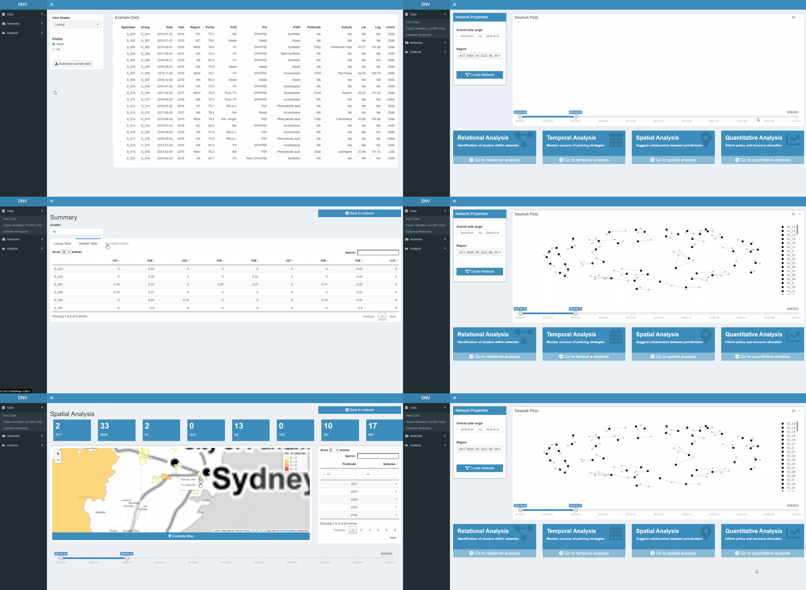
Please see the gif below for a quick demo (40 sec) of the app.
Scope
Currently, the types of visualisations created to support intelligence-led policing are static in nature [39, 102]; limiting the potential of the available information. To create actionable intelligence, it is important that drug markets and their features can be viewed and analysed in an interactive and dynamic way.
Usage
Data
This section allow users to explore the simulated data and optimise it in preparation for network visualisation. For more background information about the concepts explored in the subsequent subsections please refer to this repository.
View Data
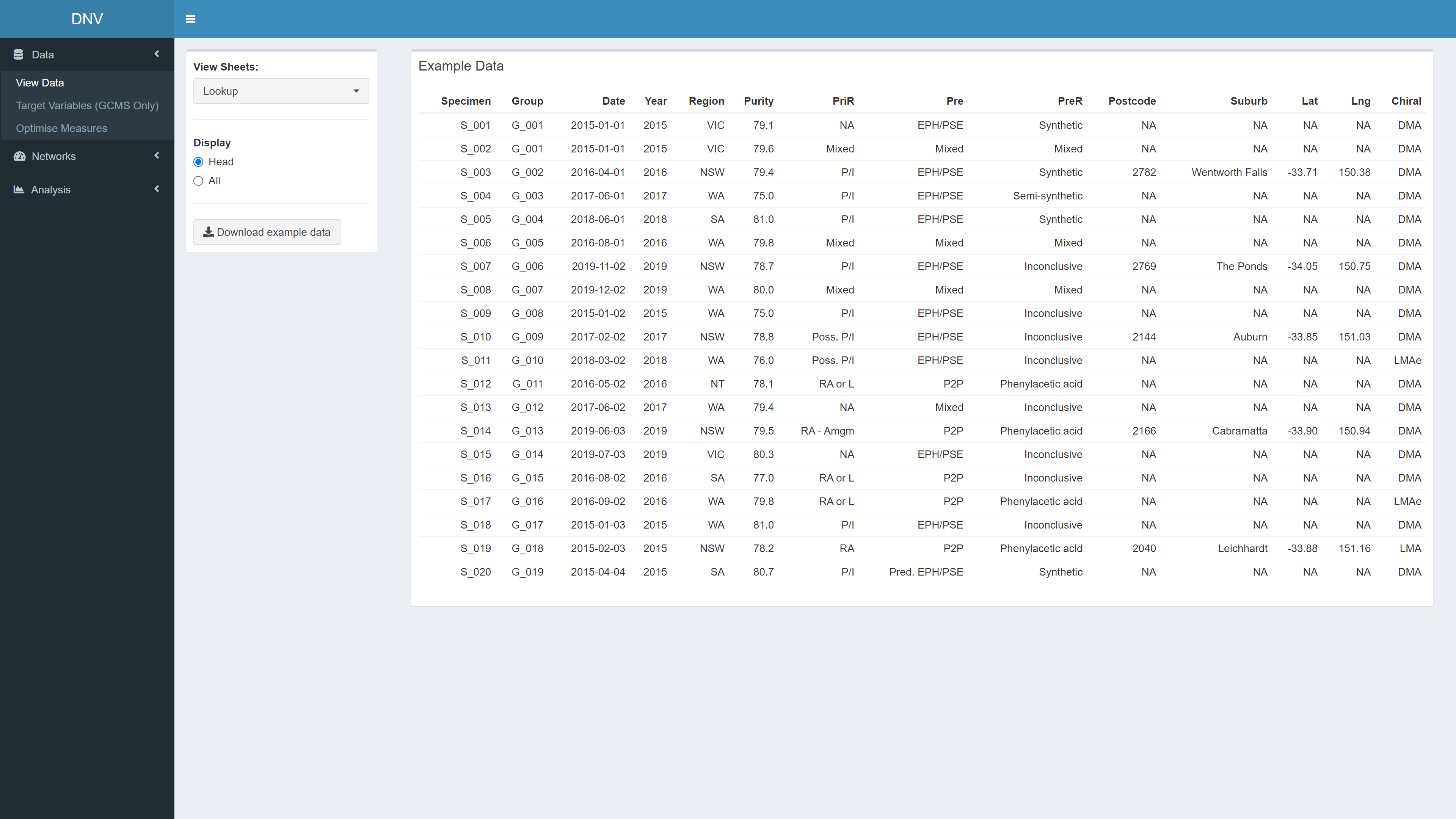
The “View Data” page is the first thing you see when the app is loaded, see Figure 1. Here you can explore and download the simulated dataset. The respective code reads in an excel file with four sheets. The first sheet is a “lookup table” with information about each specimen (i.e. seizure number, date of seizure, purity, etc.), the other three sheets relate to different profiles that have been extracted for each specimen. These profiles have been extracted using several analytical techniques; gas chromatography-mass spectrometry (GMCS), isotope-ratio mass spectrometry (IRMS) and capillary electrophoresis (CE).
Figure 1: Exploring datasets used in this project
Target Variables
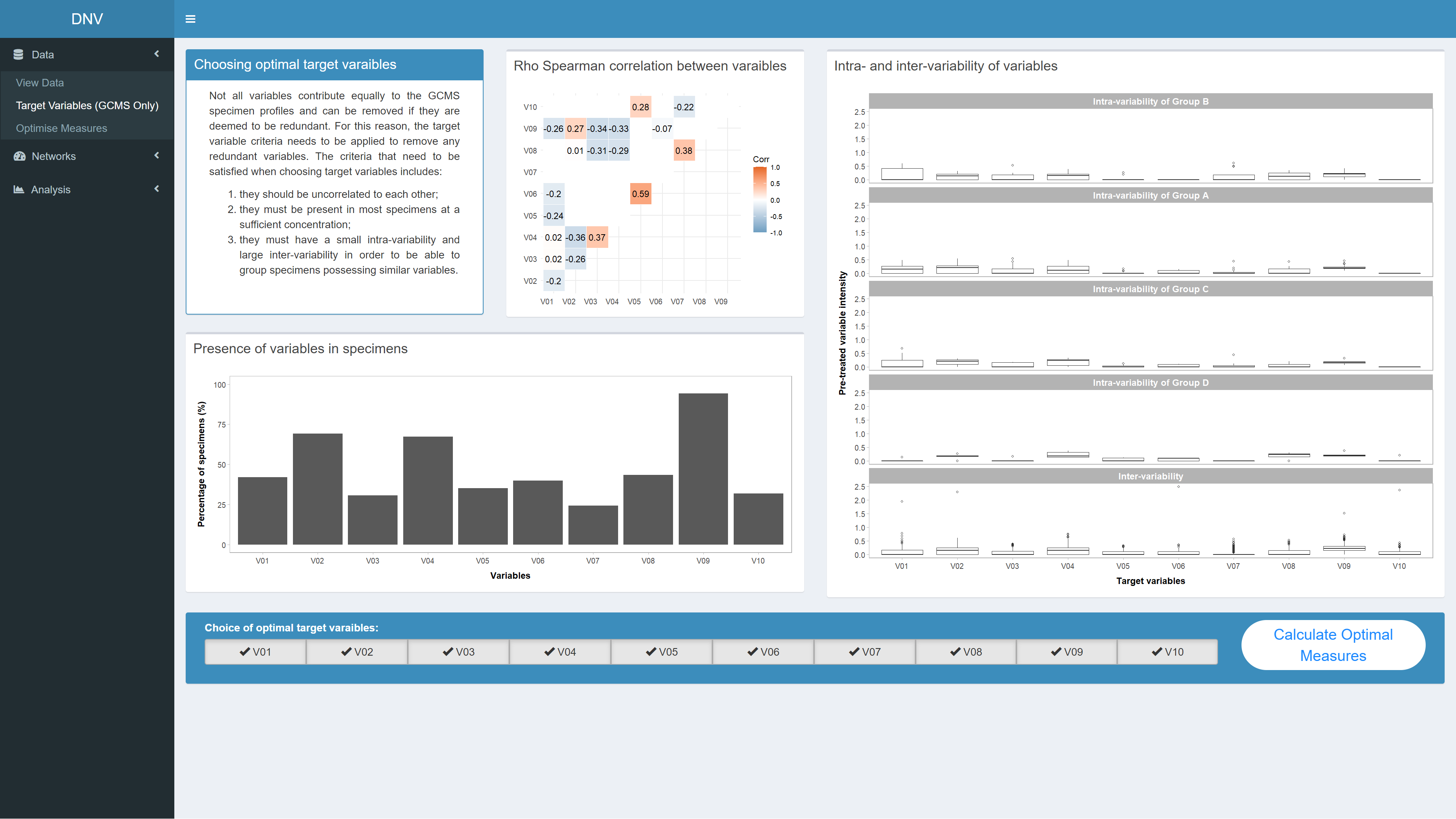
This page allows you to reduce any redundant variables in the GCMS dataset. Not all variables contribute equally to the GCMS specimen profiles and should be removed if they are deemed to be redundant. Redundant variables are identified by following the three-fold criteria on the page. Once these variables have been identified, they can be unchecked at the bottom of the page, see Figure 2. Clicking the “calculate optimal measures” button will only keep the checked target variables for subsequent analysis and also take you to the next page.
Figure 2: Reducing target variables for a particular dataset
Optimise Measures
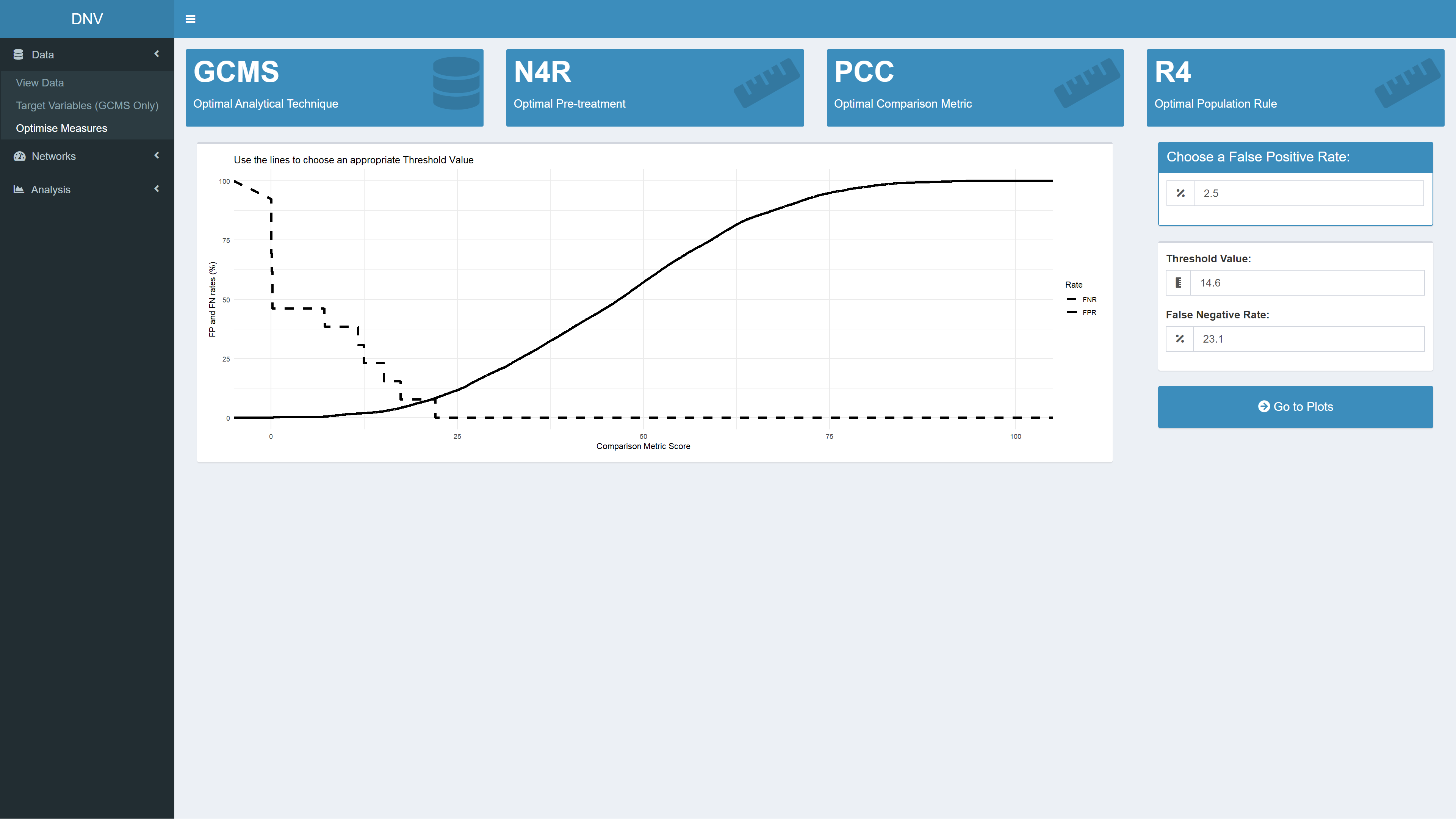
At the top of this page are several value boxes displaying optimal measures; the most discriminatory analytical technique, the optimal pre-treatment (PT), the optimal comparison metric (CM) and the optimal population rule (PR). Changing the desired target variables will affect the output of these value boxes as several PTs, CMs and PRs are tested across the three profile types (i.e. GCMS, IRMS and CE).
This page also allows users to define an acceptable threshold value (THV) for determining whether specimens are linked or not; this will influence how the network plot will look. Essentially, as the THV is decreased the number of links in the subsequent network plot will be increased. The THV can be assessed based on false positive (FP) and false negative (FN) rates of receiver operating characteristic curves, see Figure 3. In the field of forensic intelligence, a FP rate of 2.5 % is commonly acceptable. Once an acceptable FPR has been defined, the “Go to plots” button unsurprisingly takes you to the network plot.
Figure 3: Defining a threshold value for specimen linkage
Networks
This section allows users visualise illicit drug markets and review important information regarding selected network nodes.
Plots
This page allows users to plot networks between specimens and the
clusters they belong to (calculated through hierarchical clustering
analysis). As the clustering is performed on a chemical profiles of the
illicit drug specimens, the resultant clusters are referred to as
chemical classes (CC). Do to the large number of specimens, trying to
plot the relationship between CCs and specimen results in a messy graph.
A cleaner alternative is plotting the relationships between CCs and the
seizure that the specimen came from, see pane B in Figure 4.
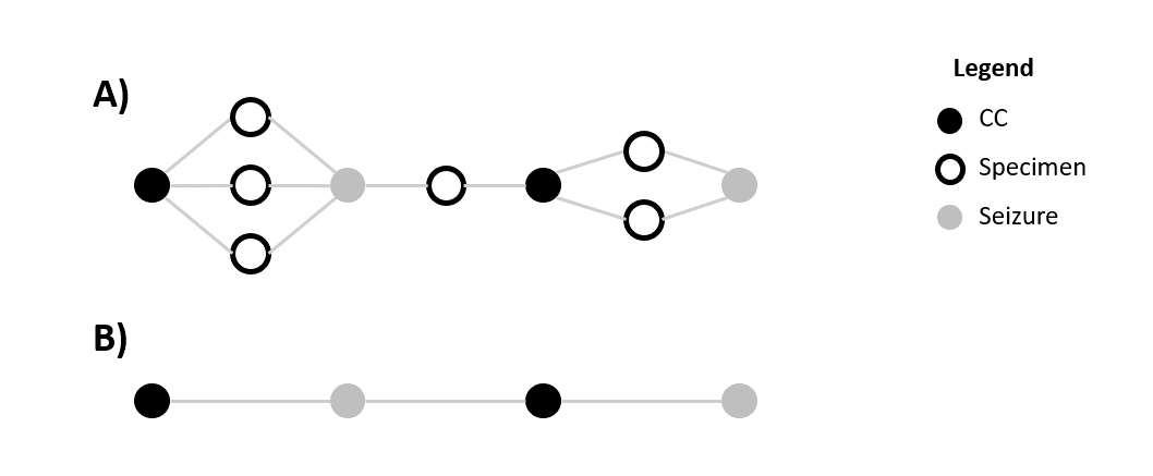
Figure 4: Relationships between CCs, specimens and seizures
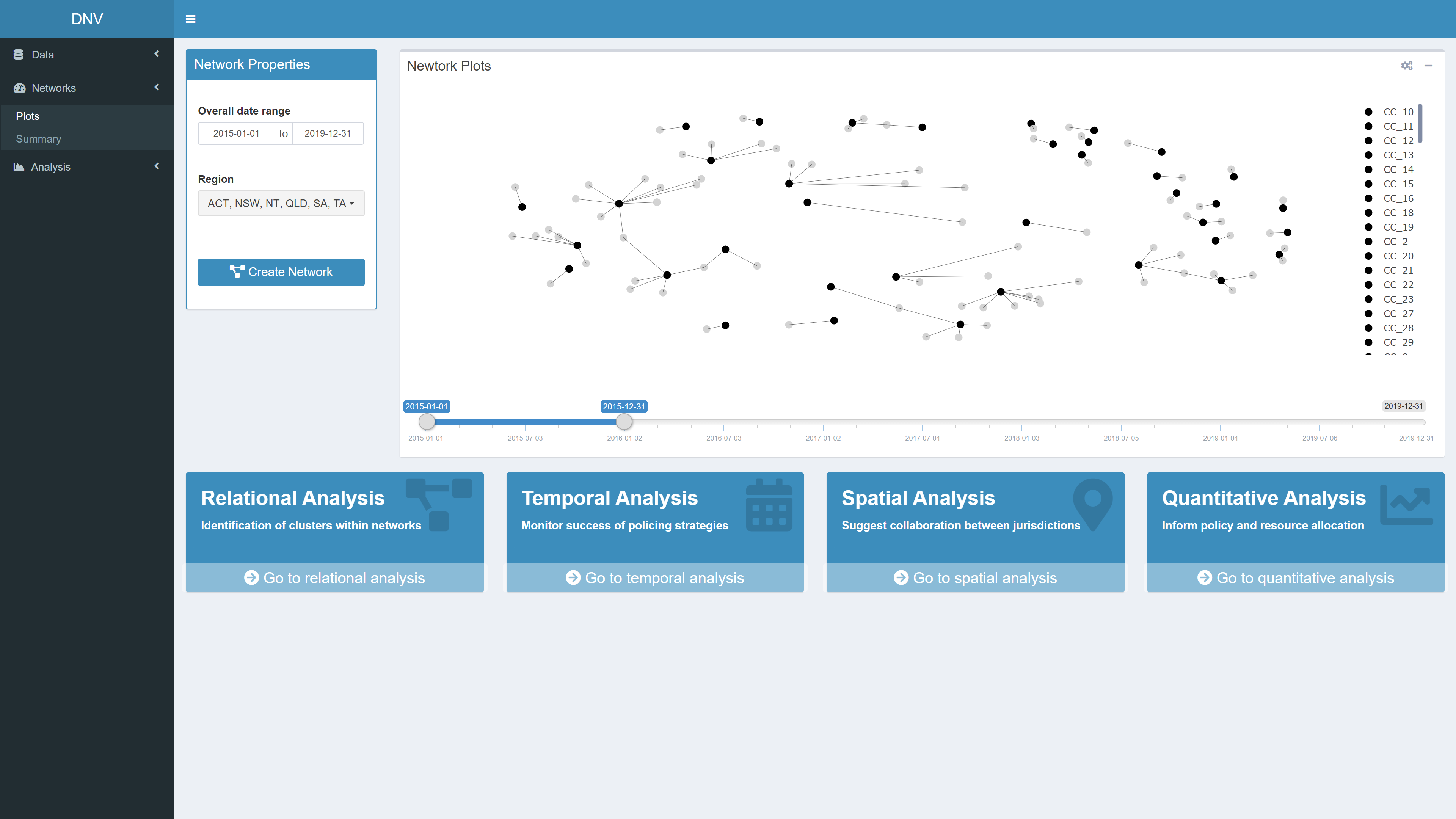
Figure 5 displays what the generated network plot looks like in the app. Users may only want to explore networks of illicit drug markets for specific date ranges or regions. For this reason the network properties should be specified before the plot is generated. The four boxes at the bottom of the page are buttons which will navigate you to the respective analysis page.
Figure 5: Network plot between specimen seizures (grey circles) and their respective CCs (black circles)
Summary
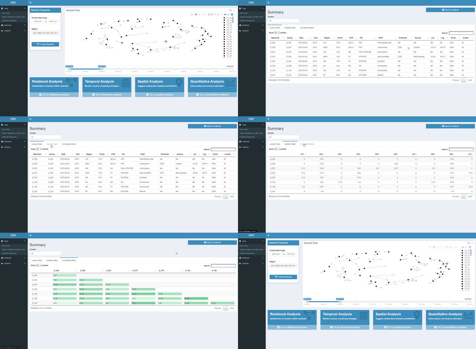
As the name suggests this page provides a summary about nodes in the active network plot, specifically it reacts to the selection of CC nodes (black circles). Information will be filtered to reflect the date range slider, regions specifed and CC selected. The information that is displayed is a subset of the lookup table, the GCMS dataset and a colour coded correlation matrix showing the similarity between specimens in the selected CC, please see the gif below for a quick demo (8 sec) of the summary page.
Analysis
This section allows users to perform relational, temporal, spatial and other quantitative analysis on illicit drug markets. For more background information about the concepts explored in the subsequent subsections please refer to this repository.
Relational Analysis
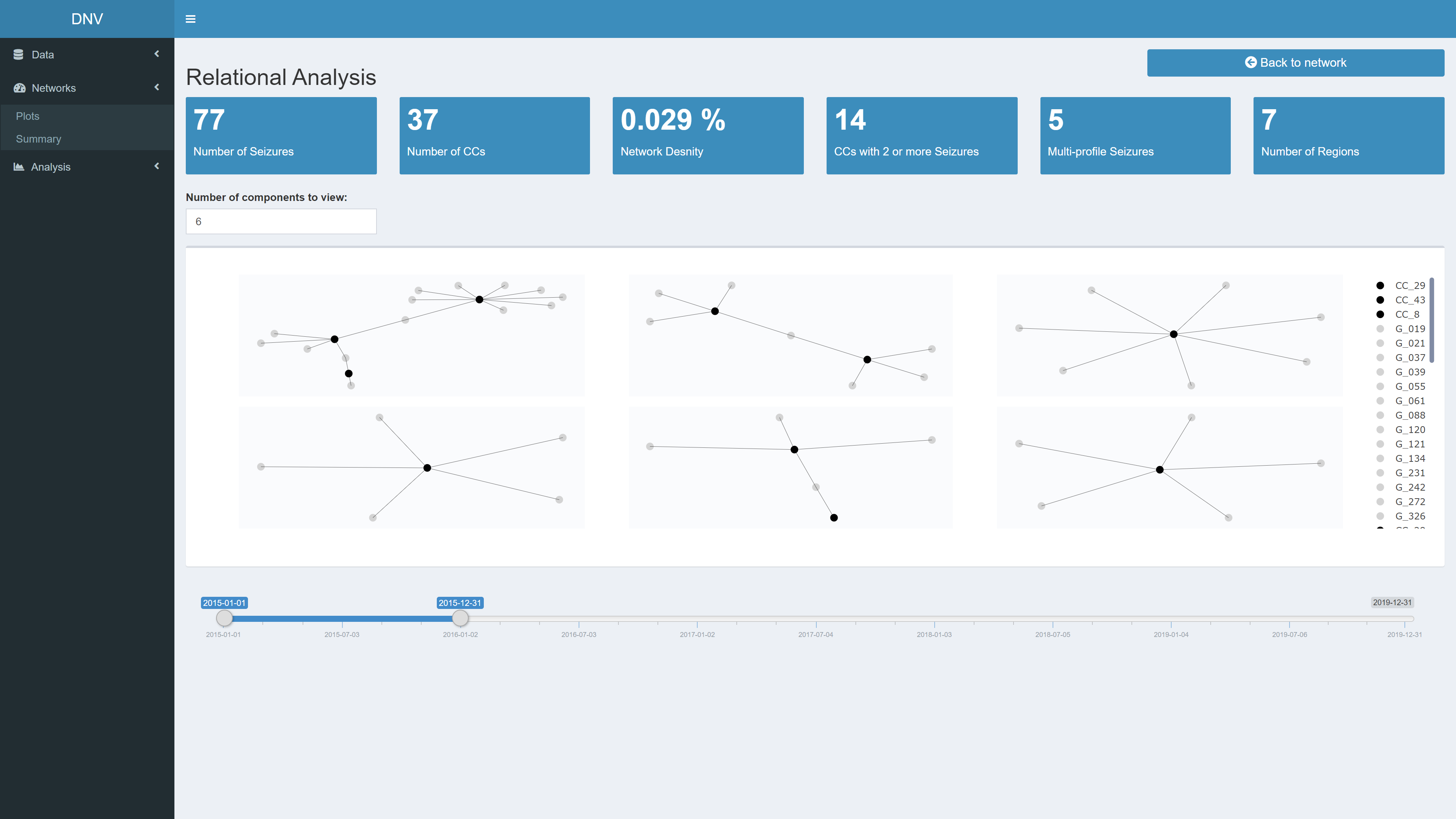
The top of the page contains several value boxes containing network measures specific to the selected date range, see Figure 6. The bottom of the page plots the n largest components in the active network. The number input above the plot controls how many “largest” components are extracted. A major part of relational analysis is identifying interesting clusters in the network, for example large components.
Figure 6: Relational analysis of active network
Temporal Analysis
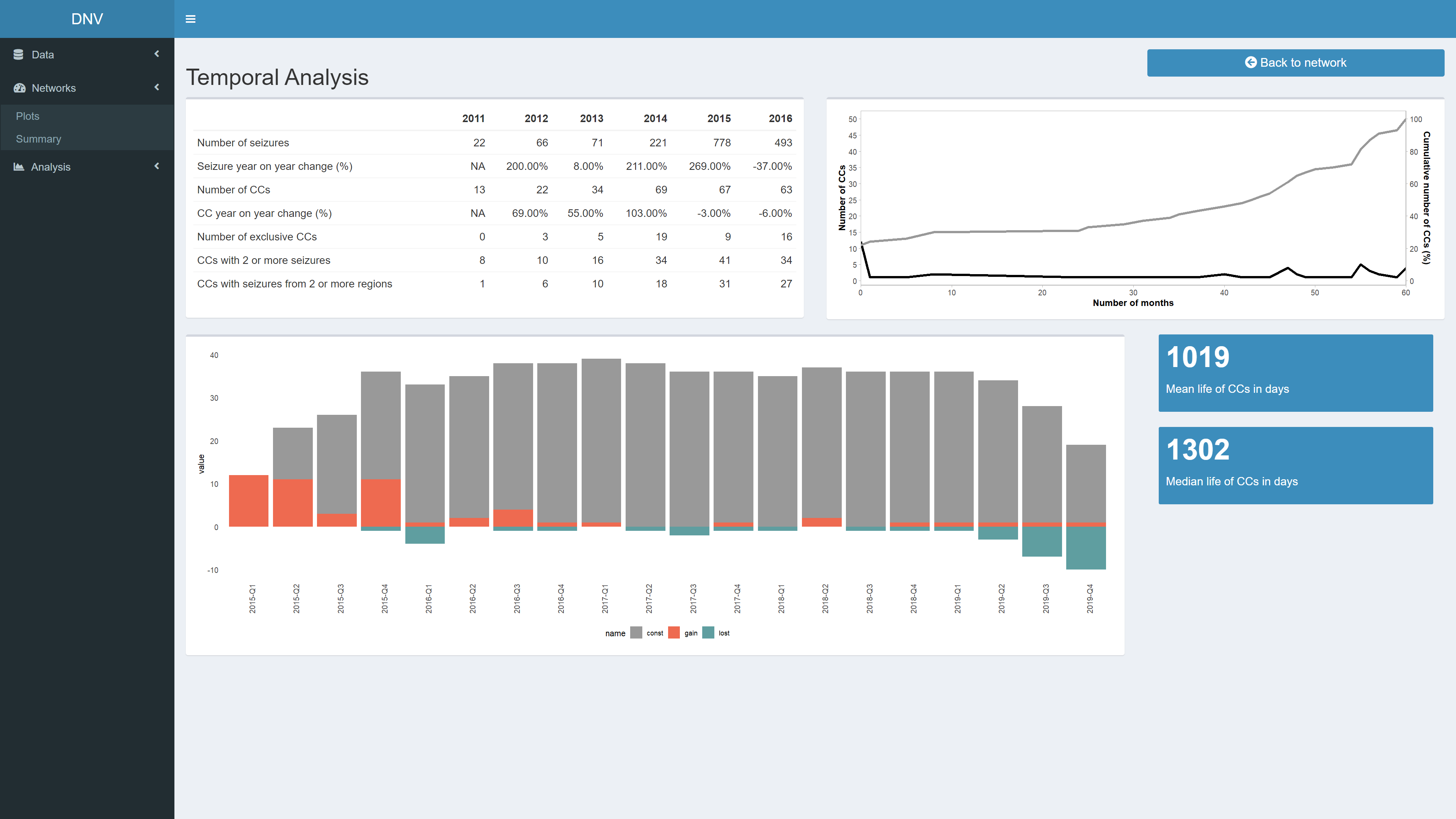
This page is not reactive to the date range sliders, instead it displays temporal measures for the entirety of the dataset. In this manner users can identify peaks in the evolution of drug markets. For example, the two value boxes in the bottom right corner display information about mean and median CC life, see Figure 7. Using this information, it would be worthwile to further investigate CCs that are observed in the network for a period longer than the mean lifetime.
Figure 7: Temporal analysis of entire network
Spatial Analysis
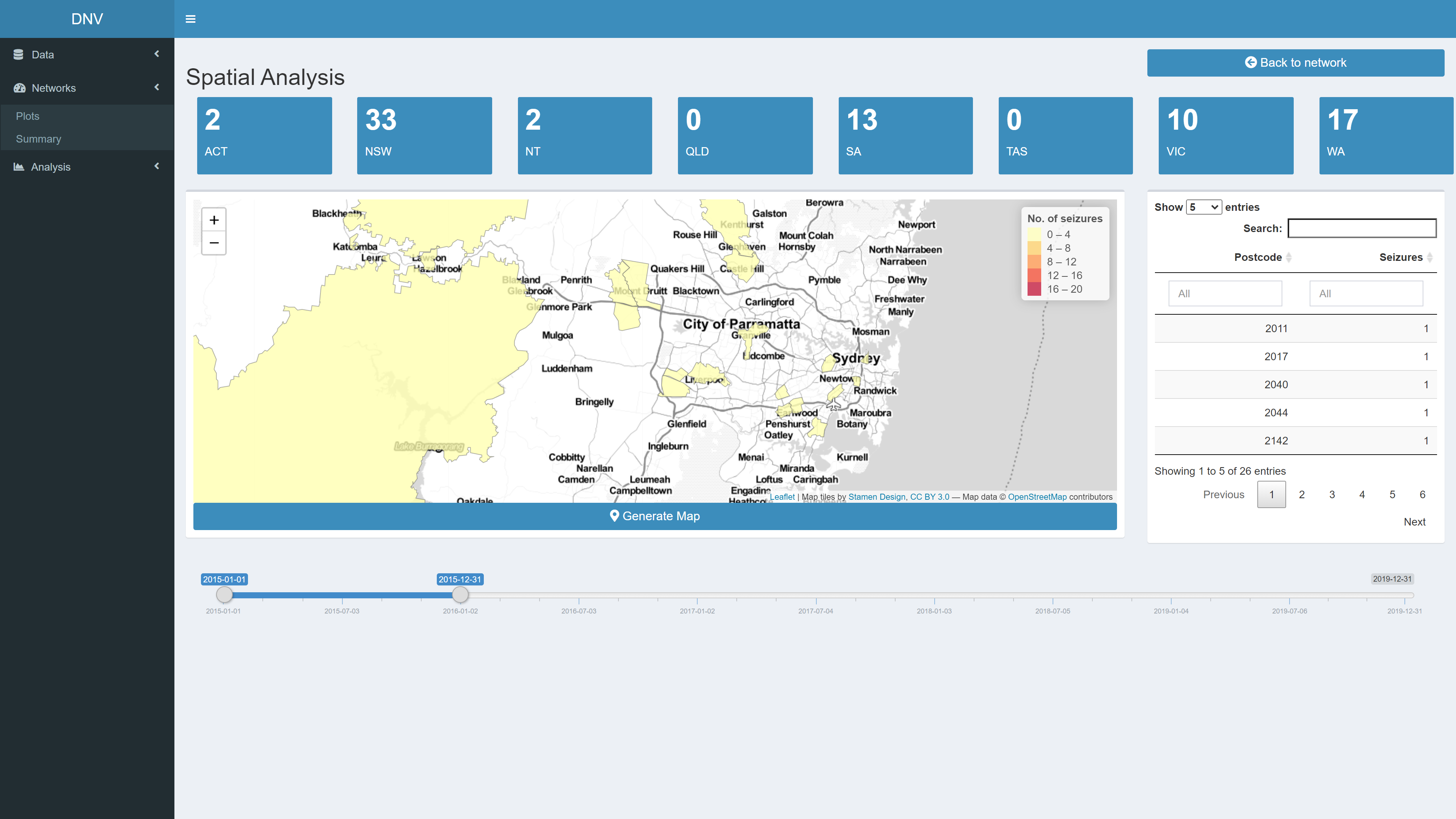
The top of the page displays the number of seizures, in the active network, from each region. The map on the bottom left of the page displays the postcodes where the seizures occured; the map is reactive to the date range slider, see Figure 7. The table on the bottom right summarises all the postcodes in the map and the number of seizures made in each. Spatial analysis of illicit drug markets is useful in suggesting where collaboration is needed between jurisdictions.
Figure 8: Relational analysis of active network
Quantitative Analysis
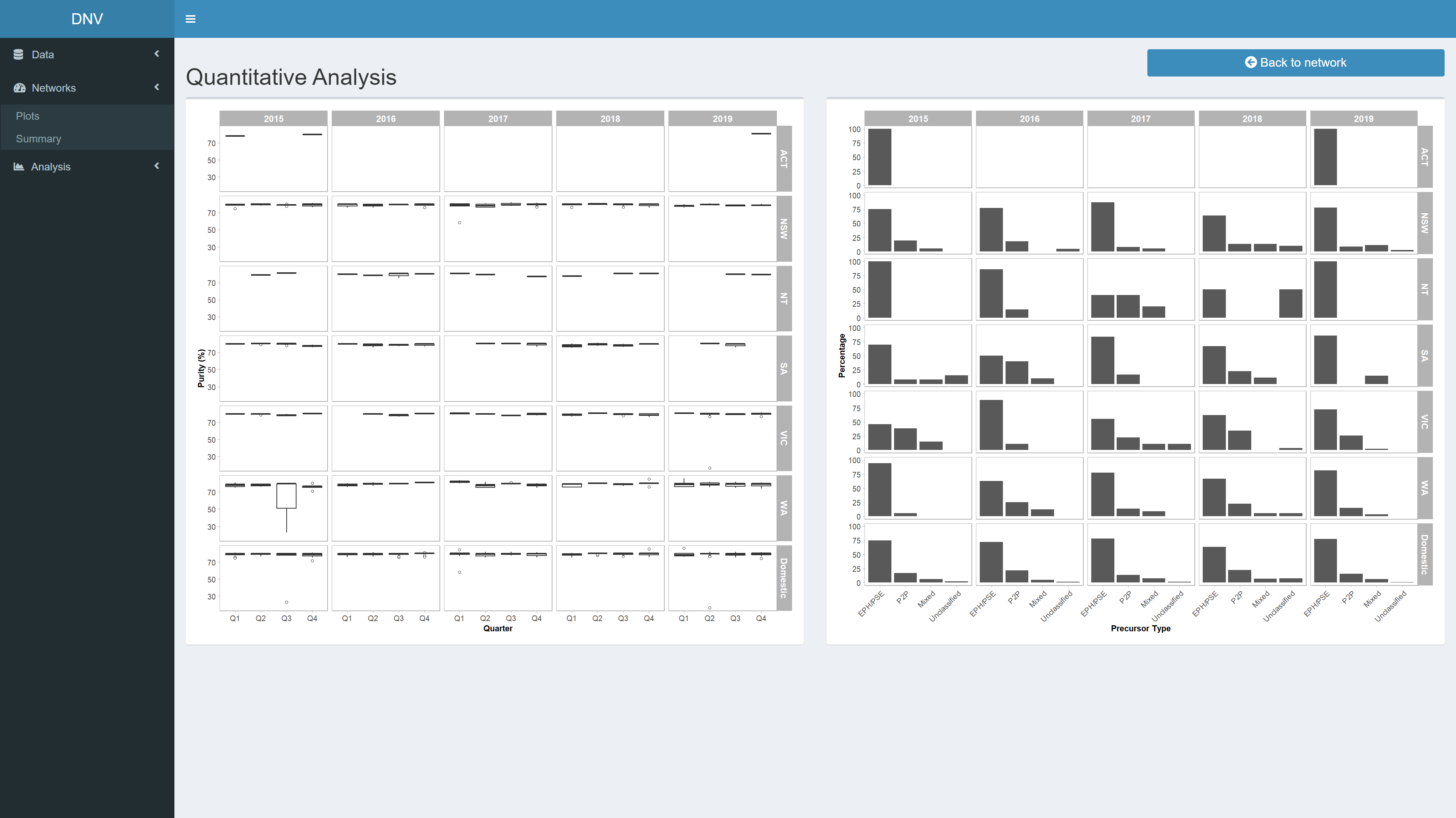
This page is not reactive to the date range sliders, instead it displays further quantitative measures for the entirety of the dataset, specifically relating to specimen purity and precursors. When quantitative data is available on drug markets, it can be evaluated in a spatiotemporal manner to analyse features of these markets and their implications for intelligence-based control measures and drug policy.
Figure 9: Relational analysis of active network
Future direction
- Allow users to upload their own datasets
- After adjusting the date range slider, adding colour to new nodes in the network plot to inform users
- Minor layout modifications
Author
Ana Popovic - popovicana
Acknowledgements
This project is part of a Australian Research Council grant (LP160100352)
This application would not be possible without key packages by other authors in the R community.
