This GitHub repository contains a sample C# console application named TOM_CreateFabricDataset which demonstrates how to automate the creation of a DirectLake-mode dataset for Power BI using the Tabular Object Model (TOM). Inside this repository, there is also a Fabric notebook named CreateLakehouseTables.ipynb with Python code which can be used to generate Lakehouse tables in delta format that will be used as the underlying datasource for the DirectLake dataset.
This document will take you through the steps required to set up and run through the demo. If you are just looking to understand how to write C# code using the Tabular Object Model (TOM), you should read CodeWalkthrough.md.
Here are the high-level steps to set up and run through this demonstration:
- Create a new workspace associated with Fabric capacity
- Create a new Fabric lakehouse in the new workspace
- Generate lakehouse tables using pre-provided Python code in Fabric notebook
- Set up and run the custom C# application to automate the creation of a DirectLake datatset
This document will now examine each of these steps in more detail.
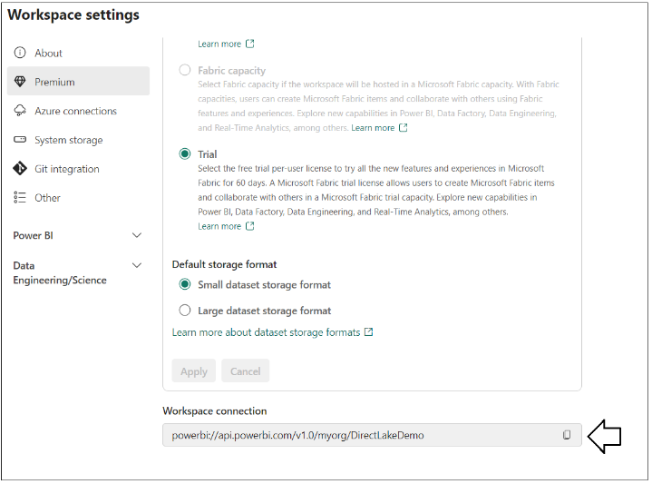
Create a new workspace with a name such as DirectLakeDemo. Make sure the workspace is associated with a Premium capacity or a Fabric trial capacity which provides Fabric capabilities. After creating the new workspace named DirectLakeDemo, select the Workspace settings menu command to display the Workspace settings pane.
In Workspace settings, select the Premium tab in the left navigation and scroll down to locate the Workspace connection setting. Click the Copy button to copy the Workspace connection string to the Windows clipboard.
As you can see, the Workspace connection string starts with powerbi:// and ends with the workspace name.
powerbi://api.powerbi.com/v1.0/myorg/DirectLakeDemo
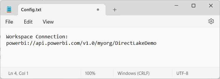
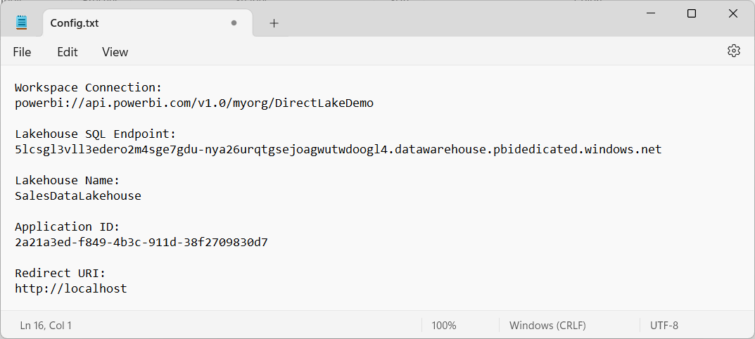
Create a new text file using Notepad.exe to save configuration data you will need later when configuring the C# console application. Copy the Workspace connection string into the text file as shown in the following screenshot.
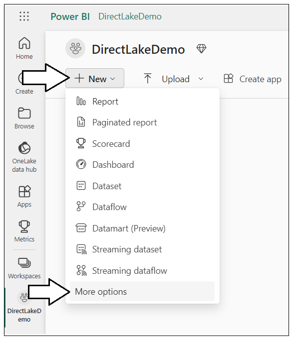
Inside the new workspace, it is time to create a new lakehouse named SalesDataLakehouse. Start by dropping down the + New menu button and select More options.
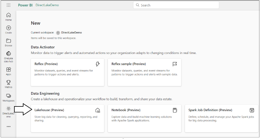
On the New page select Lakehouse (Preview) from Data Engineering section.
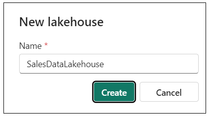
When prompted, enter a name of SalesDataLakehouse for the new Lakehouse and click Create.
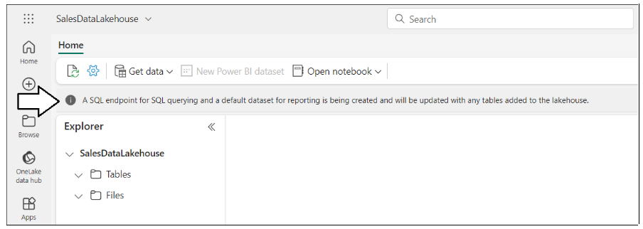
Once you have created the lakehouse, you will notice a message indicating a SQL Endpoint is being created.
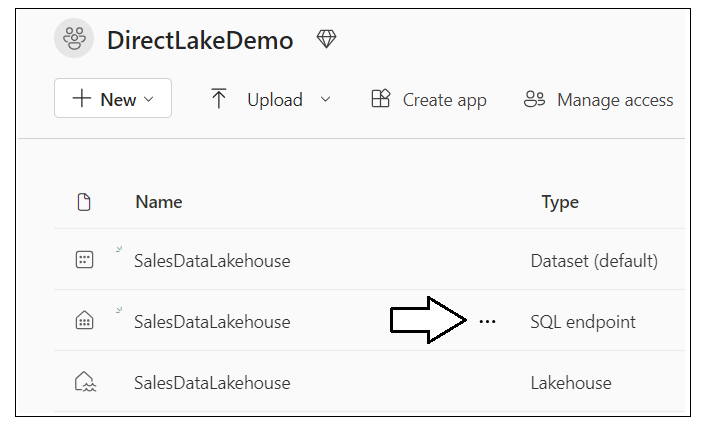
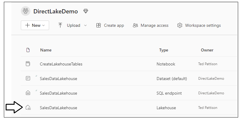
Navigate back to the main page for the DirectLakeDemo workspace. In the list of workspace items, you should see a new item for the new SQL endpoint in addition to the item for the Lakehouse. Both the Lakehouse and the SQL endpoint have the same name which is SalesDataLakehouse. Drop down the context menu for the SQL endpoint named SalesDataLakehouse.
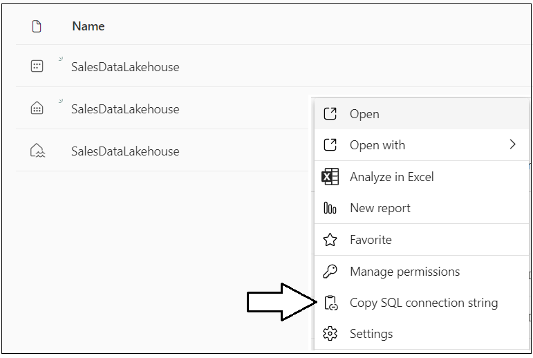
Select the Copy SQL connection string menu command from the context menu of the SQL endpoint.
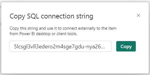
In the Copy SQL connection string dialog, click Copy to copy the connection string value to the Windows clipboard.
The connection string starts with a lakehouse identifier and ends with
.datawarehouse.pbidedicated.windows.net.
5lcsgl3vll3edero2m4sge7gdu-nya26urqtgsejoagwutwdoogl4.datawarehouse.pbidedicated.windows.net
Copy the values for the SQL endpoint and the name of the Lakehouse into the text file with configuration values as shown in the following screenshot.
Save the text file with these use these configuration values for later use when setting up the C# console application.
In this step you will import a Fabric notebook with pre-provided Python code. You will execute Python code in this notebook to populate the SalesDataLakehouse with data using a medallion architecture in which the data is stored in three data zones including a bronze zone, a silver zone and a gold zone.
In a real-world scenario, you will typcially create a seperate lakehouse for each zone. This demo is using a single lakehouse for all three zones just to simplify things and to reduce the complexity as you begin working with Python and Spark.
Start by downloading all the sources files from this GitHub repository as a single ZIP archive named TOM_CreateFabricDataset.zip. You can download the ZIP archive by clicking this link.
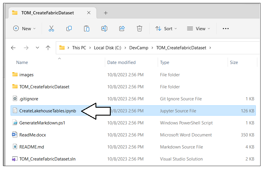
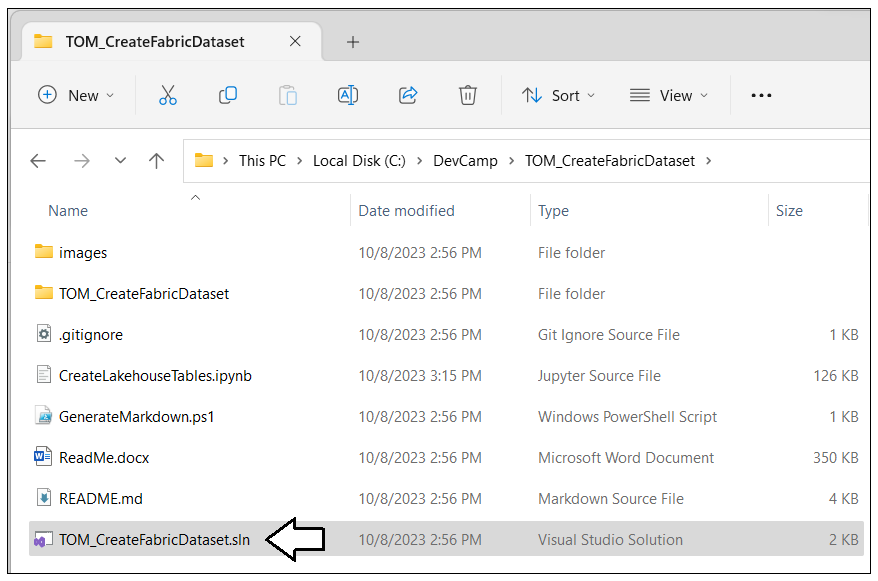
Once you have downloaded the ZIP archive named TOM_CreateFabricDataset.zip, extract the files from inside into a local folder on your machine. The screenshot below shows what the folder should look like with the extracted files. The first file you will use is a Fabric notebook with Python code named CreateLakehouseTables.ipynb.
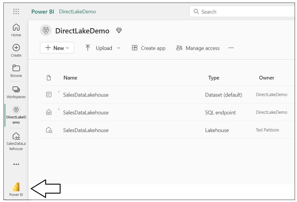
Return to the browser and navigate to the main page of the DirectLakeDemo workspace. Locate and click on the Fabric Experience Switcher menu on the bottom right of the main workspace page.
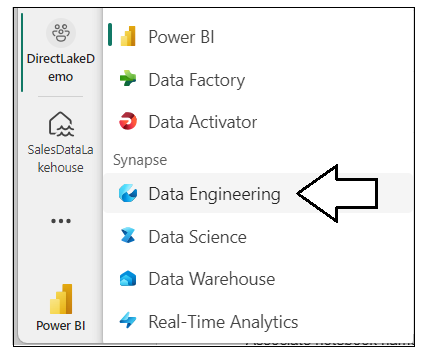
Select Data Engineering from the Fabric Experience Switcher menu.
Once you switch to the Data Engineering experience, locate and click on the Import notebook button.
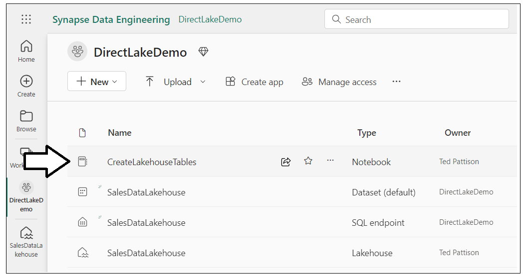
Upload Python notebook named CreateLakehouseTables.ipynb. After the notebook has been imported, you should be able to see an item for it on main workspace page. Click on CreateLakehouseTables.ipynb to open this Fabric notebook in the browser.
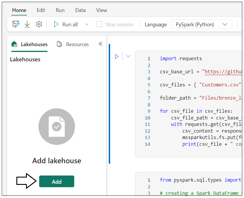
Once the notebook opens, you should be able to verify that it is not yet associated with a lakehouse. Click the Add button in the Lakehouses pane.
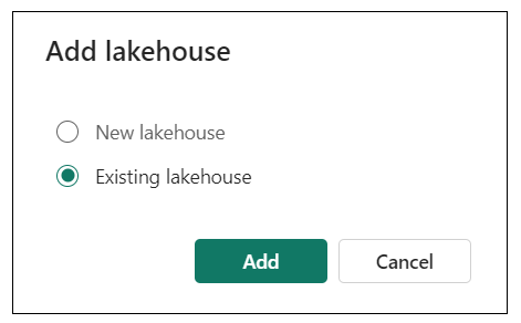
In the Add lakehouse dialog, select Existing lakehouse and click Add.
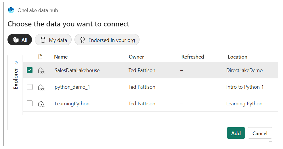
Select the lakehouse you created earlier named SalesDataLakehouse and click Add.
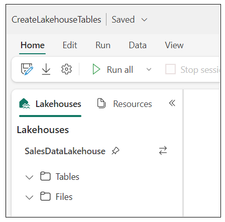
Once you have associated the notebook with the lakehouse named SalesDataLakehouse, you should see the Tables folder and the Files folder in the Lakehouses pane which are both initially empty.
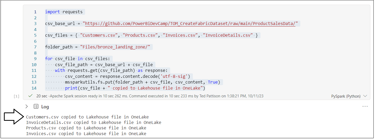
Now you will execute the Python code from this workbook to populate the lakehouse with data. You will execute the Python code in each of the notebook’s cell one by one from top to bottom. You will begin by executing Python code to copy four CSV files from this GitHub repository into the file system of the lakehouse.
Examine the following Python code in the top notebook cell which copies dour CSV files into the file system of the lakehouse.
# copy CSV files into lakehouse to load data into bronze zone
import requests

csv_base_url = "https://github.com/PowerBiDevCamp/TOM_CreateFabricDataset/raw/main/ProductSalesData/"

csv_files = { "Customers.csv", "Products.csv", "Invoices.csv", "InvoiceDetails.csv" }

folder_path = "Files/bronze_landing_zone/"

for csv_file in csv_files:
    csv_file_path = csv_base_url + csv_file
    with requests.get(csv_file_path) as response:
        csv_content = response.content.decode('utf-8-sig')
        mssparkutils.fs.put(folder_path + csv_file, csv_content, True)
        print(csv_file + " copied to Lakehouse file in OneLake")
Execute the code in the top notebook cell by clicking the Execute button located on top just to the left of the cell.
The first time you execute Python code from a Fabric notebook, it typically takes 10-20 seconds to start up and initialize the Spark pool which is used to process notebook code execution requests. When the Python code completes its execution, you'll see a message for each of the CSV files as they're copied into the lakehouse file system.
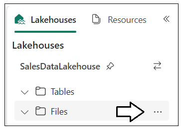
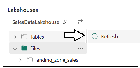
In the Lakehouses pane on the left, drop down the context menu for the Files folder.
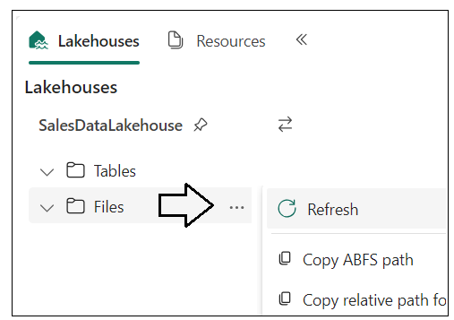
Select the Refresh command from the context menu of the Files folder.
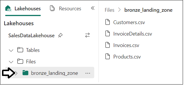
After the refresh operation completes, you should see a new child folder inside the Files folder named landing_zone_sales. If you select the landing_zone_sales folder in the left pane, you should be able to see four new CSV files named Customers.csv, InvoiceDetails.csv, Invoices.csv and Products.csv on the right.
At this point, you have now copied the CSV files with the raw data into the lakehouse file system. Now you will use Spark to load this data into memory as DataFrames where the data can be validated with table schemas and saved as lakehouse tables in delta format for the silver zone.
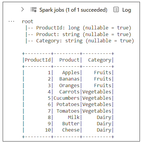
Examine the following Python code from the second notebook cell which loads product data from Products.csv into a Spark DataFrame. After the DataFrame has been loaded into memory, it is then saved as a delta table with the name silver_products. The last two lines of Python code call printSchema() and show() to display the table schema and sample rows of data below which allows you to visualize the strucutre of the product data.
# create products table for silver zone
from pyspark.sql.types import StructType, StructField, StringType, LongType, FloatType

# create schema for products table using StructType and StructField
schema_products = StructType([
    StructField("ProductId", LongType() ),
    StructField("Product", StringType() ),
    StructField("Category", StringType() )
])

# Load CSV file into Spark DataFrame and validate data using schema
df_products = (
    spark.read.format("csv")
         .option("header","true")
         .schema(schema_products)
         .load("Files/bronze_landing_zone/Products.csv")
)

# save DataFrame as lakehouse table in Delta format
( df_products.write
             .mode("overwrite")
             .option("overwriteSchema", "True")
             .format("delta")
             .save("Tables/silver_products")
)

# display table schema and data
df_products.printSchema()
df_products.show()
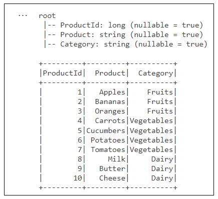
Execute the code in the second cell to load product data into a Spark DataFrame and save it as a delta table in the silver zone. After the code completes, you should see output which displays the table schema and 10 rows of product data.
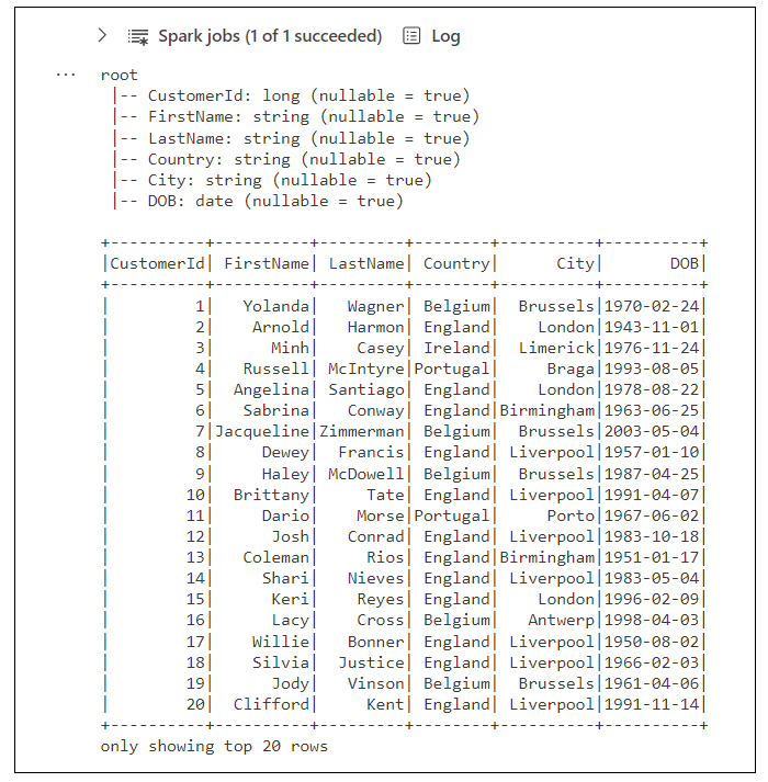
Examine the Python code inside the third cell which loads customer data from Customers.csv into a Spark DataFrame and then saves it as a delta table in the silver zone named silver_customers. You should notice this code provides special treatment to load data from a CSV file that coantains dates. More specifically, the DataFrame schema defines the DOB column using DateType() and there is code which sets two important options named dateFormat and inferSchema before calling load().
# create customers table for silver zone
from pyspark.sql.types import StructType, StructField, StringType, LongType, DateType

# create schema for customers roducts table using StructType and StructField
schema_customers = StructType([
    StructField("CustomerId", LongType() ),
    StructField("FirstName", StringType() ),
    StructField("LastName", StringType() ),
    StructField("Country", StringType() ),
    StructField("City", StringType() ),
    StructField("DOB", DateType() ),
])

# Load CSV file into Spark DataFrame with schema and support to infer dates
df_customers = (
    spark.read.format("csv")
         .option("header","true")
         .schema(schema_customers)
         .option("dateFormat", "MM/dd/yyyy")
         .option("inferSchema", "true")
         .load("Files/bronze_landing_zone/Customers.csv")
)

# save DataFrame as lakehouse table in Delta format
( df_customers.write
              .mode("overwrite")
              .option("overwriteSchema", "True")
              .format("delta")
              .save("Tables/silver_customers")
)

# display table schema and data
df_customers.printSchema()
df_customers.show()
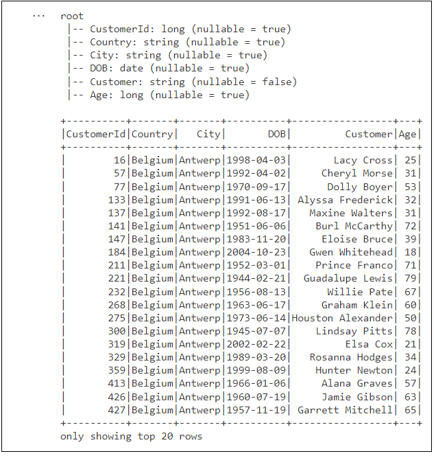
Execute the code to load customer data into a Spark DataFrame and save it as a delta table named silver_customers. After the code completes, you should see output which displays the table schema and the top 20 rows of data.
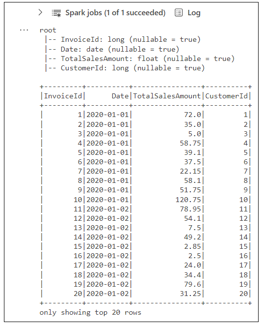
Examine the Python code in the next cell which loads invoice data from Invoices.csv into a Spark DataFrame and then saves it as a delta table in the silver zone named silver_invoices. You should notice this code provides special treatment to load data that contains dates similar to the code which creates the silver_customers table.
# create invoices table for silver zone
from pyspark.sql.types import StructType, StructField, LongType, FloatType, DateType

# create schema for invoices table using StructType and StructField
schema_invoices = StructType([
    StructField("InvoiceId", LongType() ),
    StructField("Date", DateType() ),
    StructField("TotalSalesAmount", FloatType() ),
    StructField("CustomerId", LongType() )
])

# Load CSV file into Spark DataFrame with schema and support to infer dates
df_invoices = (
    spark.read.format("csv")
         .option("header","true")
         .schema(schema_invoices)
         .option("dateFormat", "MM/dd/yyyy")
         .option("inferSchema", "true")
         .load("Files/bronze_landing_zone/Invoices.csv")
)

# save DataFrame as lakehouse table in Delta format
( df_invoices.write
             .mode("overwrite")
             .option("overwriteSchema", "True")
             .format("delta")
             .save("Tables/silver_invoices")
)

# display table schema and data
df_invoices.printSchema()
df_invoices.show()
Execute the code to load invoice data into a Spark DataFrame and save it as a delta table named silver_invoices. After the code completes, you should see output which displays the table schema and the top 20 rows of data.
Examine the Python code in the next cell which loads invoice detail data from InvoiceDetails.csv into a Spark DataFrame and then saves it as a delta table in the silver zone named silver_invoice_details.
# create invoice_details table for silver zone
from pyspark.sql.types import StructType, StructField, LongType, FloatType

# create schema for invoice_details table using StructType and StructField
schema_invoice_details = StructType([
    StructField("Id", LongType() ),
    StructField("Quantity", LongType() ),
    StructField("SalesAmount", FloatType() ),
    StructField("InvoiceId", LongType() ),
    StructField("ProductId", LongType() )
])

# Load CSV file into Spark DataFrame and validate data using schema
df_invoice_details = (
    spark.read.format("csv")
         .option("header","true")
         .schema(schema_invoice_details)
         .load("Files/bronze_landing_zone/InvoiceDetails.csv")
)

# save DataFrame as lakehouse table in Delta format
( df_invoice_details.write
                    .mode("overwrite")
                    .option("overwriteSchema", "True")
                    .format("delta")
                    .save("Tables/silver_invoice_details")
)

# display table schema and data
df_invoice_details.printSchema()
df_invoice_details.show()
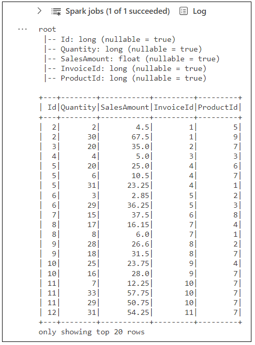
Execute the code to load invoice detail data into a Spark DataFrame and save it as a delta table named silver_invoice_details. After the code completes, you should see output which displays the table schema and the top 20 rows of data.
At this point you have created four tables which completes the work required for the silver zone.
Click the Refresh context menu of the Tables folder.
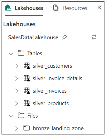
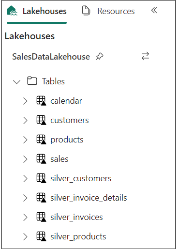
Once the refresh operation completes, you should be able to see the four tables created for the silver zone.
At this point, you have created delta tables for the silver zone which represents cleansed data with valid datatypes. In the next step, you will load silver zone tables and perform transformations to enrich the data used to create gold zone tables.
Move to the next cell which creates the products table for gold zone. This code loads the table named silver_products and then saves the data to a second delta table in the gold zone named products. Note this Python code is simple in that it does not perform any transformations on product data. However, this Python code demonstrates the basic pattern of loading a table into a DataFrame and then saving it back into lakehouse storage as a delta table with another name or in a different lakehouse.
# create products table for gold zone
# load DataFrame from silver zone table
df_gold_products = (
    spark.read
         .format("delta")
         .load("Tables/silver_products")
)

# write DataFrame to new gold zone table
( df_gold_products.write
                  .mode("overwrite")
                  .option("overwriteSchema", "True")
                  .format("delta")
                  .save("Tables/products")
)

# display table schema and data
df_gold_products.printSchema()
df_gold_products.show()
Execute the code to create the products table. After the code completes, you should see output which displays the DataFrame schema and displays the top 20 rows of data from the products table.
Move to the next cell which creates the customers table for gold zone. This code loads data from the silver_customers table and transforms the data by creating two new columns named Customer and Age. It also drops two other columns named FirstName and LastName. After performing these transformations, the code saves the DataFrame as a new table for the gold zone named Customers.
# create customers table for gold zone
from pyspark.sql.functions import concat_ws, floor, datediff, current_date, col

# load DataFrame from silver zone table and perform transforms
df_gold_customers = (
    spark.read
         .format("delta")
         .load("Tables/silver_customers")
         .withColumn("Customer", concat_ws(' ', col('FirstName'), col('LastName')) )
         .withColumn("Age",( floor( datediff( current_date(), col("DOB") )/365.25) ))
         .drop('FirstName', 'LastName')
)

# write DataFrame to new gold zone table
( df_gold_customers.write
                   .mode("overwrite")
                   .option("overwriteSchema", "True")
                   .format("delta")
                   .save("Tables/customers")
)

# display table schema and data
df_gold_customers.printSchema()
df_gold_customers.show()
Execute the code to create the customers table. After the code completes, you should see output which display the DataFrame schema and displays the top 20 rows of data from the customers table.
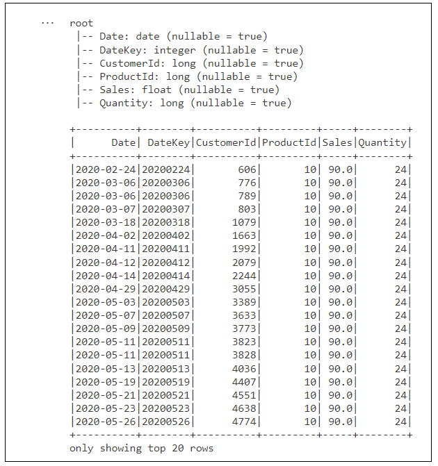
Move to the next cell which creates the sales table for gold zone. This code merges columns from the silver_invoices table and the silver_invoice_details table into a single DataFrame by calling join(). After that, this code performs several other transformations including renaming a column, generating an integer-based DateKey column, dropping unneeded columns and rearranging the order of columns.
# create sales table for gold zone
from pyspark.sql.functions import col, desc, concat, lit, floor, datediff
from pyspark.sql.functions import date_format, to_date, current_date, year, month, dayofmonth

# load DataFrames using invoices table and invoice_details table from silver zone
df_silver_invoices = spark.read.format("delta").load("Tables/silver_invoices")
df_silver_invoice_details = spark.read.format("delta").load("Tables/silver_invoice_details")

# perform join to merge columns from both DataFrames and transform data
df_gold_sales = (
    df_silver_invoice_details
        .join(df_silver_invoices,
              df_silver_invoice_details['InvoiceId'] == df_silver_invoices['InvoiceId'])
        .withColumnRenamed('SalesAmount', 'Sales')
        .withColumn("DateKey", (year(col('Date'))*10000) +
                               (month(col('Date'))*100) +
                               (dayofmonth(col('Date')))   )
        .drop('InvoiceId', 'TotalSalesAmount', 'InvoiceId', 'Id')
        .select('Date', "DateKey", "CustomerId", "ProductId", "Sales", "Quantity")
)

# write DataFrame to new gold zone table
( df_gold_sales.write
               .mode("overwrite")
               .option("overwriteSchema", "True")
               .format("delta")
               .save("Tables/sales")
)

# display table schema and data
df_gold_sales.printSchema()
df_gold_sales.show()
Execute the code to create the sales table. After the code completes, you should see output which display the DataFrame schema and displays the top 20 rows of data from the sales table.
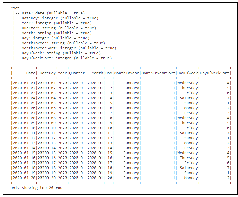
Move down to the last cell which creates the calendar table in the gold zone which is used for time-based analysis. If you examine the code, you can see it retrieves the first date and last date from the Date column of the sales table to determine where to start and to end the calendar table. There is also code to add several calculated columns to the calendar table such as Year, Quarter, Month, Day, MonthInYear and DayOfWeek. Finally, note the code creates a calculated column named DateKey that will be used to establish a one- to-many relationship between the calendar table and the sales table.
# create calendar table for gold zone
from datetime import date
import pandas as pd
from pyspark.sql.functions import to_date, year, month, dayofmonth, quarter, dayofweek, date_format

# get first and last calendar date from sakes table
first_sales_date = df_gold_sales.agg({"Date": "min"}).collect()[0][0]
last_sales_date = df_gold_sales.agg({"Date": "max"}).collect()[0][0]

# calculate start date and end date for calendar table
start_date = date(first_sales_date.year, 1, 1)
end_date = date(last_sales_date.year, 12, 31)

# create pandas DataFrame with Date series column
df_calendar_ps = pd.date_range(start_date, end_date, freq='D').to_frame()

# convert pandas DataFrame to Spark DataFrame and add calculated calendar columns
df_calendar_spark = (
     spark.createDataFrame(df_calendar_ps)
       .withColumnRenamed("0", "timestamp")
       .withColumn("Date", to_date(col('timestamp')))
       .withColumn("DateKey", (year(col('timestamp'))*10000) +
                              (month(col('timestamp'))*100) +
                              (dayofmonth(col('timestamp')))   )
       .withColumn("Year", year(col('timestamp'))  )
       .withColumn("Quarter", date_format(col('timestamp'),"yyyy-QQ")  )
       .withColumn("Month", date_format(col('timestamp'),'yyyy-MM')  )
       .withColumn("Day", dayofmonth(col('timestamp'))  )
       .withColumn("MonthInYear", date_format(col('timestamp'),'MMMM')  )
       .withColumn("MonthInYearSort", month(col('timestamp'))  )
       .withColumn("DayOfWeek", date_format(col('timestamp'),'EEEE')  )
       .withColumn("DayOfWeekSort", dayofweek(col('timestamp')))
       .drop('timestamp')
)

# write DataFrame to new gold zone table
( df_calendar_spark.write
                   .mode("overwrite")
                   .option("overwriteSchema", "True")
                   .format("delta")
                   .save("Tables/calendar")
)

# display table schema and data
df_calendar_spark.printSchema()
df_calendar_spark.show()
Execute the code to create the calendar table. After the code completes, you should see output which display the DataFrame schema and displays the top 20 rows of data from the calendar table.
Now refresh the Tables folder in the Lakehouses pane. You should now see the four gold zone tables named calendar, customers, products and sales. These are the delta tables that will be used to create the DirectLake-mode dataset.
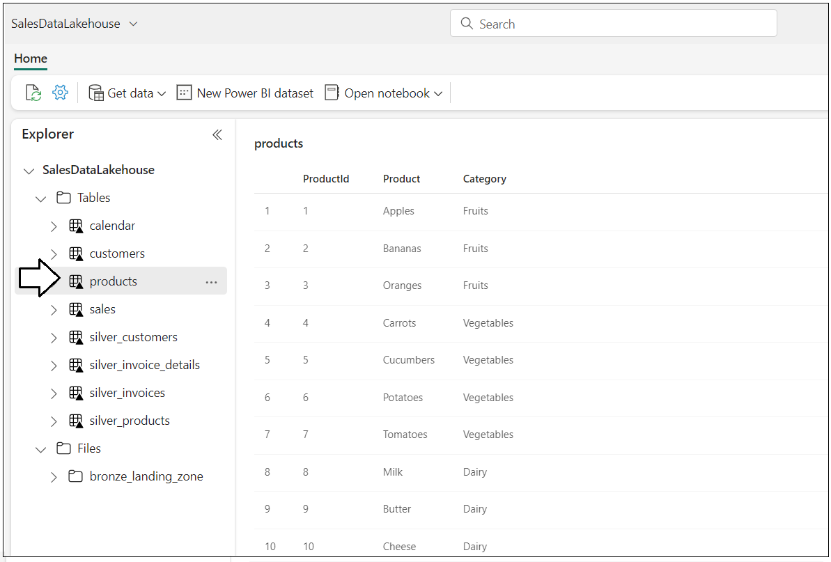
Navigate to the main page of the DirectLakeDemo workspace and then click on the workspace item for the lakehouse named SalesDataLakehouse.
Now you can see and inspect the tables in the lakehouse. Start by clicking on the products table to see its contents.
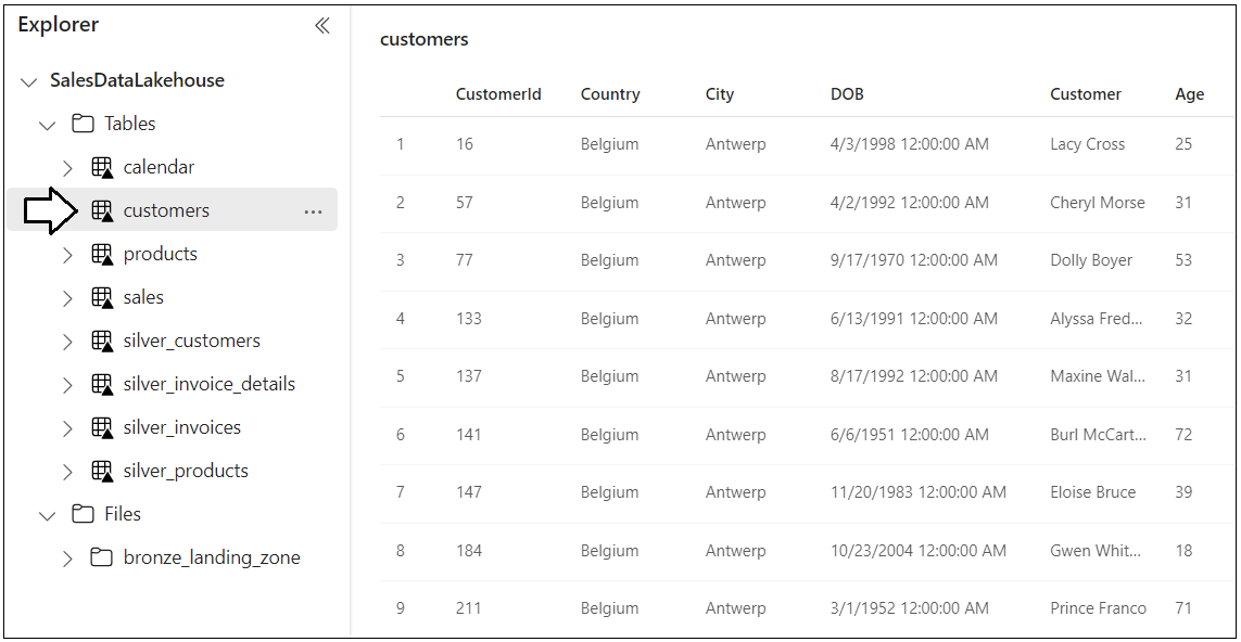
Inspect the data in the customers table.
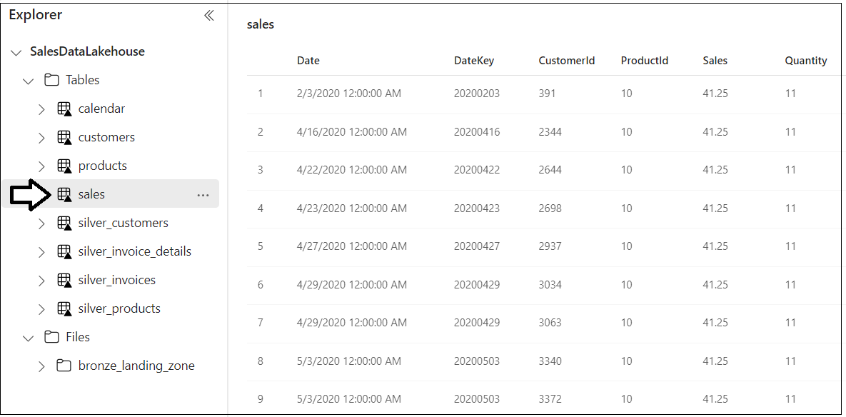
Inspect the data in the sales table.
Inspect the data in the calendar table.
Now all Lakehouse tables have been created and you can move on to the next step where you create the DirectLake dataset using the custom application with C# code.
In case you have not heard, Microsoft recently renamed Azure Active Directory to Microsoft Entra ID. In the past, you would uses the Azure AD portal to create an Azure application which can be used to call Microsoft APIs such as the Tabular Object Model. Now, you will use the Microsoft Entra admin center to create a new application for the C# console application.
In order to set up the C# console application, you must first create a new application. Start by navigating to Microsoft Entra admin center at the following URL.
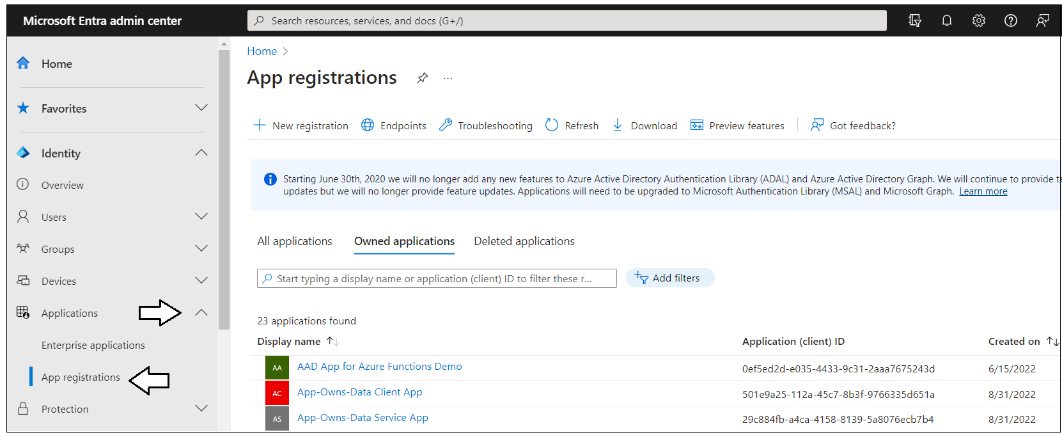
On the home page of the Microsoft Entra admin center, drop down the Applications section in the left navigation and click the App registrations link.
On the App registrations page, click New registration.
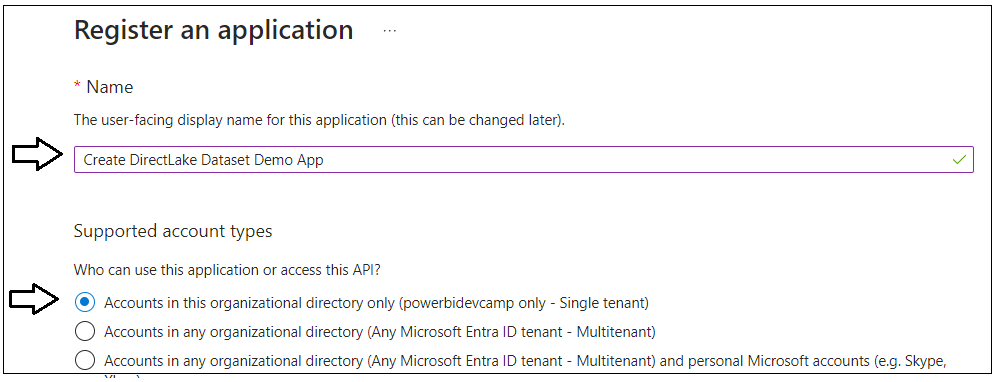
Give the new application a name such as Create DirectLake Dataset Demo App and leave the Supported account types setting with the default selection of Accounts in this organizational directory only.
Move down to the Redirect URI section. Select Public client/native application in the drop down menu and enter a redirect URI of http://localhost. Make sure to create the URL with http and not https.
Click Register to create the new application.
Now that you have created the application, you need to record Application ID for use later in the C# console application. Copy the Application ID from the application summary page in the Microsoft Entra admin center.
Add the Application ID and Redirect URI of http://localhost into the text file with configuration data.
Now you have recorded all the configuration data you need to set up and run the C# console application to create the DirectLake-mode dataset.
In an earlier step you extracted all the files from this repository into a local folder. If you examine the files in this folder, you will see a Visual Studio solution file named TOM_CreateFabricDataset.sln.
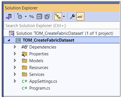
Double-click on TOM_CreateFabricDataset.sln to open the project in Visual Studio 2022. You should see the project structure as shown in the following screenshot.
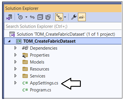
Open the C# file named AppSettings.cs so you can update configuration values used by the application.
You can see AppSettings.cs has several constants for configuration values that you need to update before running the application.
Update AppSettings.cs by adding configuration values for WorkspaceConnection, SQLEndpoint, TargetLakehouseName, ApplicationID. You should also make sure that RedirectUrl is correctly set to http://localhost.
You can optionally update AppSettings.cs with your UserId and UserPassword if you want to avoid an interactive login each time you run the application. If you leave these values blank, you will be promoted to login each time you run the application.
Save your changes to AppSettings.cs. You are now ready to run the application.
Run the application in debug mode by pressing {F5} or selecting Debug > Start Debugging.
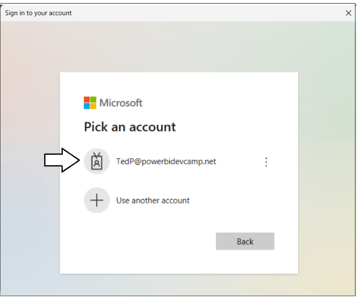
When the application starts, you will be promoted to login. Log in using the same user account you have been using throughout this demo to create the workspace and lakehouse.
After successfully logging in, wait until the program completes. It might take as long as 20-30 seconds.
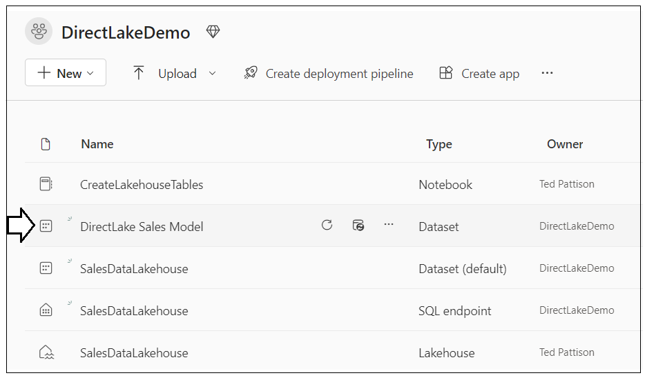
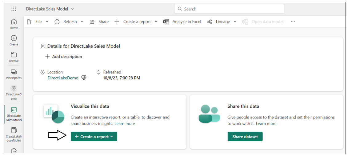
The application should run and complete without any errors. When the application completes, navigate to the home page of the DirectLakeDemo workspace and refresh the workspace page with the list of items. Verify that you can see new dataset named DirectLake Sales Model. Click on the named DirectLake Sales Model item to navigate to its details page.
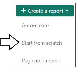
On the Details for DirectLake Sales Model page, click + Create a report to drop down this menu.
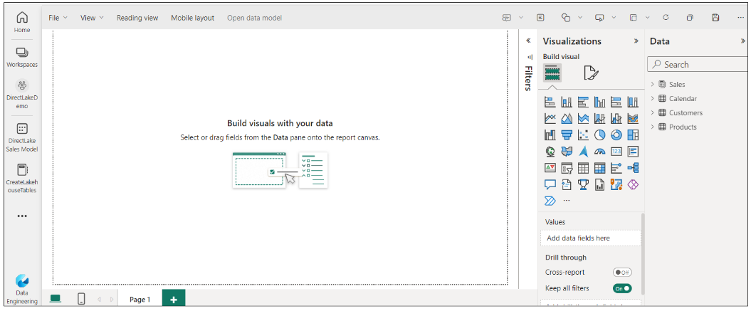
Select Start from scratch to create a new report so you can test out the new dataset.
You should now be able to build a report using this DirectLake-mode dataset.
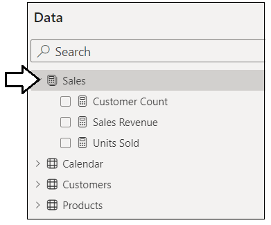
Examine the Sales table which contains three measures.
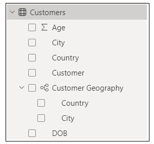
Examine the Customer table which contains several columns and a dimensional hierarchy.
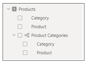
Examine the Products table which contains several columns and a dimensional hierarchy.
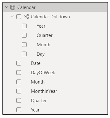
Examine the Calendar table which contains several columns and a dimensional hierarchy.
You have now generated a DirectLake-mode dataset which can be used to create Power BI reports. This is the end of the demonstration. Designing a report that looks good is left as an exercise for the reader.
While this document examined the steps required to set up and run the demo, it did not really explain how the C# code created a Direct-mode dataset using the Tabular Object Model. If you want to understand how to write C# code to create a Direct-mode dataset, you should read CodeWalkthrough.md.

