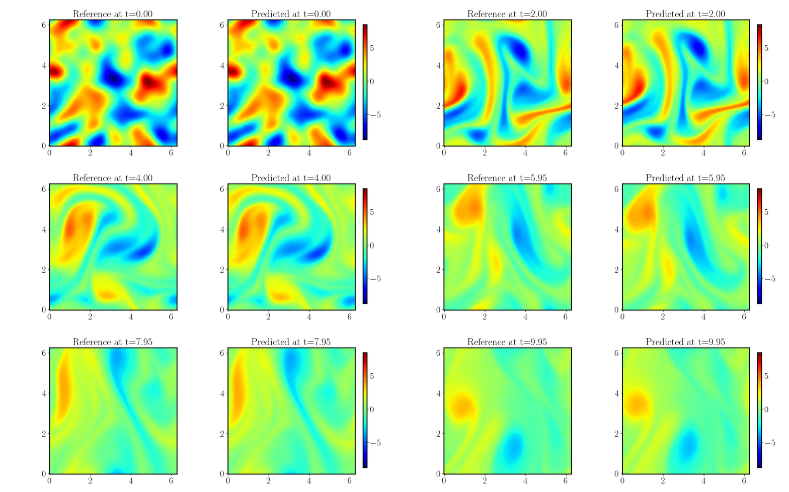
This repository is a comprehensive implementation of physics-informed neural networks (PINNs), seamlessly integrating several advanced network architectures, training algorithms from these papers
- Understanding and Mitigating Gradient Flow Pathologies in Physics-Informed Neural Networks
- When and Why PINNs Fail to Train: A Neural Tangent Kernel Perspective
- Respecting Causality for Training Physics-informed Neural Networks
- Random Weight Factorization Improves the Training of Continuous Neural Representations
- On the Eigenvector Bias of Fourier Feature Networks: From Regression to Solving Multi-Scale PDEs with Physics-Informed Neural Network
- PirateNets: Physics-informed Deep Learning with Residual Adaptive Networks
- Fourier Features Let Networks Learn High Frequency Functions in Low Dimensional Domains
- A Method for Representing Periodic Functions and Enforcing Exactly Periodic Boundary Conditions with Deep Neural Networks
- Characterizing Possible Failure Modes in Physics-Informed Neural Networks
This repository also releases an extensive range of benchmarking examples, showcasing the effectiveness and robustness of our implementation. Our implementation supports both single and multi-GPU training, while evaluation is currently limited to single-GPU setups.
- May 2024: We have released the code for our latest paper, "PirateNets: Physics-informed Deep Learning with Residual Adaptive Networks". Please see repo branch pirate for the implementation and examples.
Ensure that you have Python 3.8 or later installed on your system. Our code is GPU-only. We highly recommend using the most recent versions of JAX and JAX-lib, along with compatible CUDA and cuDNN versions. The code has been tested and confirmed to work with the following versions:
- JAX 0.4.26
- CUDA 12.4
- cuDNN 8.9
You can install the latest versions of JAX and JAX-lib with the following commands:
pip3 install -U pip
pip3 install --upgrade jax jaxlib
Install JAX-PI with the following commands:
git clone https://github.com/PredictiveIntelligenceLab/jaxpi.git
cd jaxpi
pip install .
We use Weights & Biases to log and monitor training metrics. Please ensure you have Weights & Biases installed and properly set up with your account before proceeding. You can follow the installation guide provided here.
To illustrate how to use our code, we will use the advection equation as an example.
First, navigate to the advection directory within the examples folder:
cd jaxpi/examples/advection
To train the model, run the following command:
python3 main.py
To customize your experiment configuration, you may want to specify a different config file as follows:
python3 main.py --config=configs/sota.py
Our code automatically supports multi-GPU execution.
You can specify the GPUs you want to use with the CUDA_VISIBLE_DEVICES environment variable. For example, to use the first two GPUs (0 and 1), use the following command:
CUDA_VISIBLE_DEVICES=0,1 python3 main.py
Note on Memory Usage: Different models and examples may require varying amounts of GPU memory.
If you encounter an out-of-memory error, you can decrease the batch size using the --config.batch_size_per_device option.
To evaluate the model's performance, you can switch to evaluation mode with the following command:
python3 main.py --config.mode=eval
In the following table, we present a comparison of various benchmarks. Each row contains information about the specific benchmark,
its relative
| Benchmark | Relative |
Checkpoint | Weights & Biases |
|---|---|---|---|
| Allen-Cahn equation | allen_cahn | allen_cahn | |
| Advection equation | adv | adv | |
| Stokes flow | stokes | stokes | |
| Kuramoto–Sivashinsky equation | ks | ks | |
| Lid-driven cavity flow | ldc | ldc | |
| Navier–Stokes flow in tori | ns_tori | ns_tori | |
| Navier–Stokes flow around a cylinder | - | ns_cylinder | ns_cylinder |
@article{wang2023expert,
  title={An Expert's Guide to Training Physics-informed Neural Networks},
  author={Wang, Sifan and Sankaran, Shyam and Wang, Hanwen and Perdikaris, Paris},
  journal={arXiv preprint arXiv:2308.08468},
  year={2023}
}

@article{wang2024piratenets,
  title={PirateNets: Physics-informed Deep Learning with Residual Adaptive Networks},
  author={Wang, Sifan and Li, Bowen and Chen, Yuhan and Perdikaris, Paris},
  journal={arXiv preprint arXiv:2402.00326},
  year={2024}
}


