normalweatherr is an R package to conduct meteorological/weather normalisation on air quality so trends and interventions can be investigated in a robust way.
To install the development version the devtools package will need to be installed first. Then:
# Load helper package
library(devtools)

# Install normalweatherr
install_github("davidcarslaw/normalweatherr")
-
Gain a mostly complete time-series of a numeric value with other variables which could explain variation of the numeric value. In the air quality domain,
valuewill usually be a pollutant concentration and the other variables will be meteorological variables such as wind speed, wind direction, atmospheric temperature, and atmospheric pressure. However other variables could be used which might explain pollutant concentrations. The time-series will usually be at hourly or daily resolution. -
A statistical model is built which uses meteorological and time variables to explain pollutant concentrations. Any statistical model which can represent interactions and non-linear relationships among the predictors could be used. But here, random forest (with randomForest), support vector machines (with kernlab), generalised boosted regression models (with gbm), and generalised additive models (with mgcv) are used.
-
Evaluate performance of the statistical model. Depending on the type of model and input data, this can include:
- Model performance metrics such as MSE and R<sup>2</sup>.

- Importance matrices.

- Partial dependency plots.

- Test the [bias-variance trade off](https://en.wikipedia.org/wiki/Bias%E2%80%93variance_tradeoff) by using withheld data not used in the model generation but were contained in the original set (the [training and test sets](https://en.wikipedia.org/wiki/Test_set)).
-
Randomly allocate the meteorological and time variables, but excluding the trend component used in the model to predict concentrations based on these sampled variables. When this process is repeated hundreds of times and then aggregated, the result is a prediction which represents "average" meteorology/weather.
-
Continue on with appropriate trend analysis. Breakpoints, Theil-Sen estimations, etc...
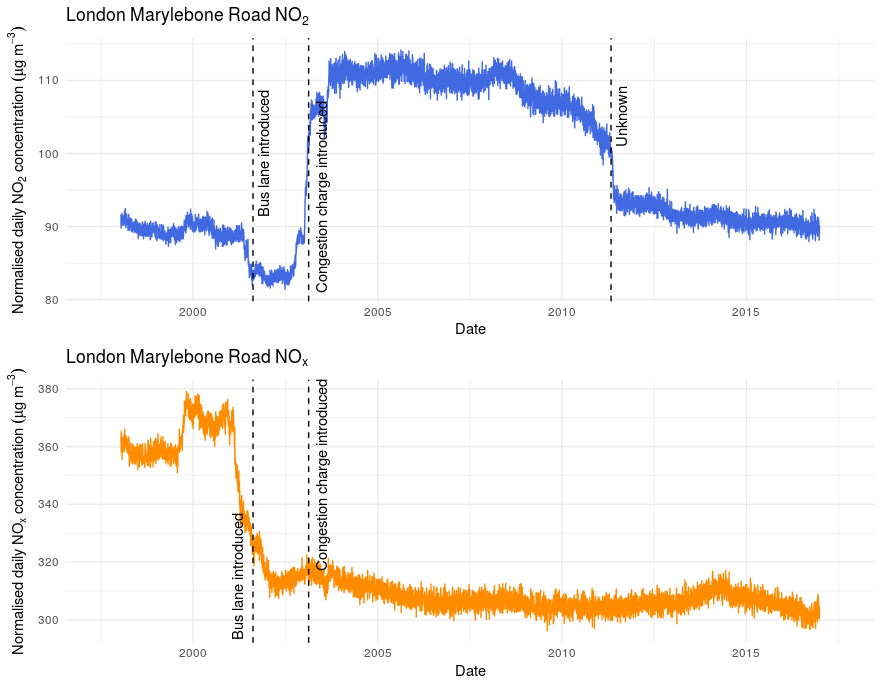
The plots below show meteorological normalised trends for NO2 and NOx at London Marylebone Road between 1997 and 2016. Due to the normalisation procedure, these plots represent the emissions at London Marylebone Road.
These trends are not suitable for formal trend tests because they are not monotonic, i.e. they are not constantly changing with time. However, the breakpoints can be explained by changes in traffic management.
NO2 shows an increase in emissions when the London congestion charge was introduced. Although this may be counter-intuitive, it can be explained by a large increase in bus traffic. Diesel buses in the early 2000s also emitted more primary NO2 than passenger cars. The reason for the abrupt decrease in May 2011 is unknown to me at the moment.
The NOx trend demonstrates that despite all the efforts gone into emission control, NOx emissions at London Marylebone Road have remained stable since the early 2000s.
After installation, this example can be run using prepared data from London Marylebone Road (NO2) and London Heathrow (the surface meteorological data). The value variable is NO2 concentration in μg m-3.
# Load packages
library(dplyr)
library(normalweatherr)
library(openair)

# Load a prepared data frame
file <- "http://skgrange.github.io/www/data/london_marylebone_road_no2_data.rds"
data_london <- readRDS(url(file))

# Look at data
glimpse(data_london)

# Make modelling reproducible
set.seed(123)

# Prepare data, add the time variables
data_london <- add_date_variables(data_london)

# and split into the training and testing sets
list_input_data <- split_input_data(data_london)

# What are the names of the sets?
names(list_input_data)

# Build model
# What variables will be used?
variables <- c("wd", "ws", "air_temp", "day_julian", "date_unix", "weekday")

# Build the random forest model
model_rf <- calculate_model(
  list_input_data,
  variables = variables,
  mtry = 3,
  nodesize = 3,
  model = "rf"
)

# Check
names(model_rf)

# Print model things
model_rf$model
# Good performance, r2 ~80 %

# Normalise for meteorology
# Implements parallel processing to speed things up

data_normalised <- normalise_for_meteorology(
  model_rf$model,
  data_london,
  variables = setdiff(variables, "date_unix"),
  n = 1000
)

# Plot normalised time series
timePlot(data_normalised, "value_predict", key = FALSE, cols = "dodgerblue")
