This repository contains all my projects for the Self-Driving Car Engineer Nanodegree at Udacity.
Brief description of what was implemented in each project. Note that many important algorithm steps and implementation details are skipped in this section. For more information about a project, please see that projects writeup.md report and where available, the Jupyter notebook.
Color thresholding and edge detection is used to extract potential lane line pixels. The Hough transform is then applied to find short straight-line segments among the extracted pixels, which are grouped together and averaged to get a straight-line approximation of the left and right lane-line. The final result is shown as overlays in the videos below.
Directory: ./term1/P1-LaneLines/
Report: writeup.md
Jupyter notebook: P1.ipynb
Video: solidWhiteRight.mp4, solidYellowLeft.mp4, challenge.mp4
A convolutional neural-network (CNN) is designed and trained to classify German traffic signs. The traffic signs are already extracted from the camera images and is presented to the algorithm as 32x32 RGB image samples. The data set contains in total 51839 examples of 43 different classes. The data is imbalanced among the classes, ranging from 180 to 1860 examples per class.
The CNN is created using Tensorflow. To simplify evaluation of different variants of the CNN, Tensorflow is wrapped into my own framework of neural-network operations, which among other things takes care of the cumbersome calculations needed for input and output sizes in each layer. In the end, it was actually possible to generate networks, which made it possible to run exhaustive searches for the best layer configuration and hyper-parameters.
Directory: ./term1/P2-Traffic-Sign-Classifier/
Report: writeup.md
Jupyter notebook: Traffic_Sign_Classifier.ipynb
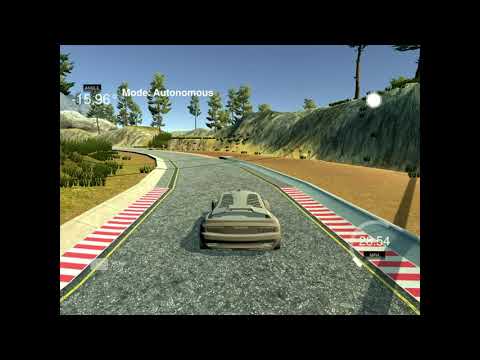
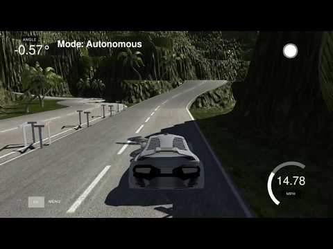
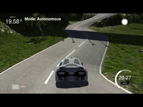
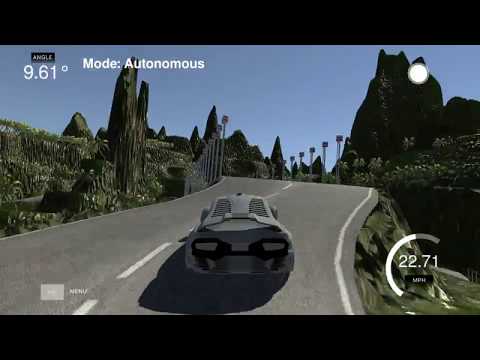
A convolutional neural-network (CNN) is trained to clone the behavior from manually driving around two different tracks in a simulator. The input to the model is the image from a forward looking mono-camera, and the output is a steering signal. For the CNN architecture in this project, I tried the network presented in this NVIDIA blog post, which actually is small enough to run in real-time on NVIDIA's embedded hardware. The training data was gathered to make the model generalize as much as possible, using both tracks, both directions and horizontally flipped images. A combination of over- and under-sampling was applied to somewhat equalize the data with respect of steering angle, shadows and road types. Additional shadow examples was also generated by augmenting track 1 data. To help the model learn how to handle situations when the vehicle starts to drift away from the center, the simulator also provides images from a left- and a right-side mounted camera, which was used together with an steering angle offset to provide lots of training data that helps the model stabilize towards the road/lane center. To make the model handle even worse driving errors, a number of recovery sequences was recorded where the vehicle started at the road side and then manually was stabilized to road/lane center.
Directory: ./term1/P3-Behavioral-Cloning/
Report: writeup.md
Video from camera view: track1 at 30 MPH, track2 at 15 MPH
Video from simulator view (of the more challenging second track):
| 15 MPH | 20 MPH | 25 MPH |
|---|---|---|
 |
 |
 |
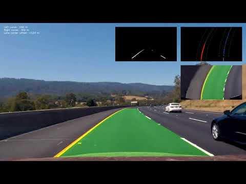
In the first lane project, the output was two straight-lines representing the left and right lane-lines in the camera image coordinates. In this project, the output is a second degree polynomial describing the lane lines in real-world coordinates. The both polynomials are then used to estimate the curvature of the lane at the vehicles current position, and also the position within the lane.
In order for this to become somewhat accurate, the distortion in the camera lens must be corrected for in the raw-camera image. For this, the algorithm relies heavily on the camera calibration functions in OpenCV, which process a set of chessboard images to find the distortion coefficients which are used in the image processing pipeline to undistort images.
Similar to the first lane-line project, potential lane-line pixels are extracted using image filters. More effort was however put into this in this project, using several different color and edge filters combined in union or intersect to produce a single output binary image. A visual tool was implemented to help develop and tune this filter. The tool dynamically generates windows for each node that is configured in the filter, and provides sliders to tune the thresholds of all leaf nodes. The thresholds can be adjusted in real-time during video playback. Here's a screenshoot of the tool.
The binary image is then transformed to bird's eye view using a pre-calculated perspective transform, such that each pixel represents a physical distance in real-world coordinates.
Two methods are implemented to do the final extraction of pixels that belongs to a lane-line, one for initial searches and the other when there are previous knowledge about the lines. A polynomial is finally fitted to the pixels belonging to a lane-line.
In the video below, the inverse perspective transform is applied in order to draw the lane detection as a green overlay in the undistorted camera image.
Directory: ./term1/P4-Advanced-Lane-Lines/
Report: writeup.md
Video:
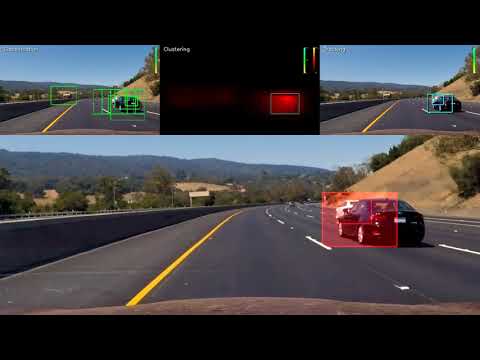
Vehicles are classified using traditional machine learning with sliding windows at different scales. The classified objects are then clustered using a heatmap image and tracked using a combination of position and size prediction, new observations and optical flow.
Directory: ./term1/P5-Vehicle-Detection-and-Tracking/
Report: writeup.md
Video:
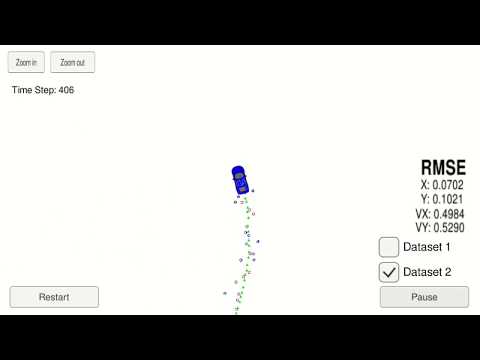
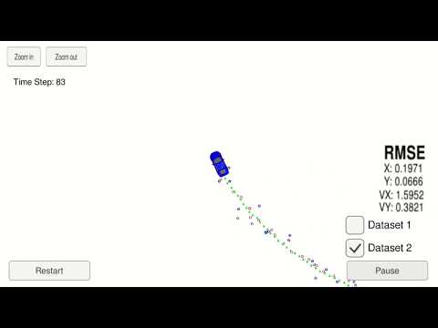
The position of an object is tracked using sensor fusion of LIDAR and RADAR measurements. The linear LIDAR measurements are processed using the standard Kalman filter. The non-linear RADAR measurements are processed using the extended Kalman filter, where the the non-linear measurement function is approximated using the Jacobian matrix.
Directory: ./term2/P6-Extended-Kalman-Filter/
Report: writeup.md
Video:
The same tracking problem as in P6. In this project, the motion model used gives non-linearity also in the prediction step and another method is used to approximate non-linearity. The "Unscented" part of the name of this method is just a goof by the inventor, who disliked the Extended Kalman filter approach to deal with non-linearity. With UKF, the approximation is instead implemented by generating sigma points that represents the probability distribution at current time-step. The sigma points are then transitioned through the non-linear function and used to calculate the probability distribution at next time-step.
Directory: ./term2/P7-Unscented-Kalman-Filter/
Report: writeup.md
Video:
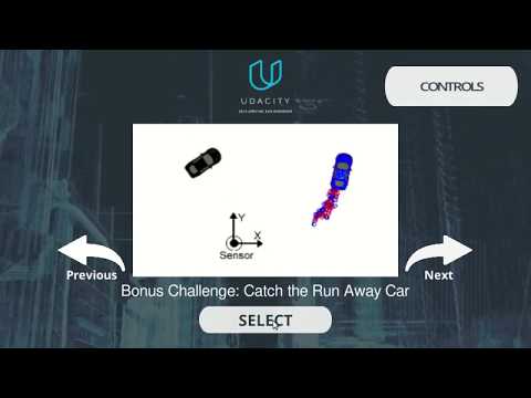
There was also a bonus challenge in this project. The UKF filter is now used to track a run away car, and the application shall steer a hunting vehicle to intercept it. The extra challenge in this is to predict the position of the run-away vehicle ahead of time, such that the hunting vehicle, although it drives at the same speed, will be able to intercept it.
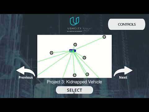
Use a particle filter to localize the position of ego vehicle given a map of landmarks and LIDAR observations of landmarks.
A particle filter generates lots of particles, which are more or less qualified guesses of the system state at time k. Then it evaluates how good each particle is based on how well it fits actual measurements of the system state. The better a particle fits the measurements, the higher is the probability that it will be represented in next iteration (when estimating the system state at time k+1).
Directory: ./term2/P8-Kidnapped-Vehicle/
Report: writeup.md
Video:
Implement a controller, that use Proportional, Integral and Derivative (PID) components to drive a vehicle around a track in a simulator environment. The simulator provides current cross-track error and velocity as input to the controller, which then shall provide steering angle and throttle/break value.
The PID coefficients was tuned using an algorithm called Twiddle, which essentially increases or decreases the coefficients one at a time, more or less aggressively in order to zoom in on the best values.
One problem with tuning the coefficients in the simulator is that when the vehicle crashes, then the simulator must be manually restarted. To work around this, a "safe mode" was implemented, in which the speed is reduced and a special PID controller instance that is good at recovering is activated.
The final controller utilize a combinations of multiple PID instances to safely drive the vehicle as fast as possible around the track.
Directory: ./term2/P9-PID-Contoller/
Report: writeup.md
Video:
Implement a controller that use Model Predictive Control (MPC) to drive a vehicle around a track in a simulator environment. The simulator provides the vehicles current position, orientation and velocity, as well as a few waypoints ahead of the vehicle that describes the track. An extra delay of 100 ms is also implemented in the control loop to mimic a real system where input sensor readings and output actuations typically not are disposed/applied without some delay.
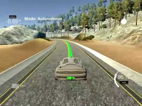
The controller implemented in this project is based on a motion model that is used to predict how the vehicle would proceed forward when given a sequence of steering and throttle actuations to be carried out at specific time-steps. The predicted path is then compared to a target path, where the crosstrack error (cte) and orientation error (epsi) is calculated and accumulated for all time-steps in the prediction. The accumulated cte and epsi are finally evaluated by a cost function, that also looks at other aspects of the predicted path such as the actuations being applied, in order to provide a scalar cost value that defines how well this prediction suits the desired behavior of the controller. Given the motion model and the cost function, an optimizer is employed to find the predicted path that have the lowest cost. The very first actuations in the most cost effective prediction is then the only output from the controller at current time-step. For the next time step, the optimization process is repeated since there is an updated state vector to consider.
The controller was tuned to safely drive the vehicle as fast as possible around the track. In the video below, note that the controller actually is straightening up the path by going wide before and then cutting through the curves, which it does on purpose to achieve higher velocity.
Directory: ./term2/P10-Model-Predictive-Control/
Report: writeup.md
Video:
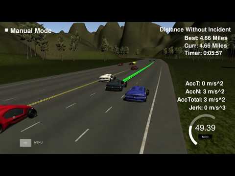
Implement a path planner for American style high-way traffic. The vehicle shall drive as fast as possible without exceeding the speed limit, colliding or choosing dangerous/confusing paths, e.g. avoid driving too close to other vehicles and keep to the center of a lane unless changing. When possible, the vehicle shall change lane in order to pass slower vehicles.
This was implemented by first generating many somewhat reasonable trajectories, that then in the next step is evaluated by cost functions to determine which one is the best.
Directory: ./term3/P11-Path-Planning/
Report: writeup.md
Video:
