RMiftakhov/PolicyGradientMethod-REINFORCE-drlnd

PolicyGradientMethod-REINFORCE-drlnd

The code is based on materials from Udacity Deep Reinforcement Learning Nanodegree Program.

Report

The policy methods are the class of RL (Reinforcement Learning) methods that do not estimate value function directly but tries to optimize the weights of the policy network that would maximize the expected return by interacting with an environment. Policy gradient methods (PGM) are a subclass of policy-based methods. PGM optimize the weights of the policy network by gradient ascent.

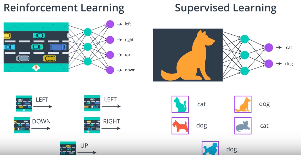
As it was noted by many, including Andrej Karpathy, that RL shares more features with Supervised Learning. The connection with Supervised learning is pretty straightforward. Supervised learning setup, we have a bunch of labeled data that is feed into NN, in this context learning means tweaking the weights (back-propagation) of the NN to identify a given picture correctly. Changing the weights increases the probability of giving the right label. In RL setup, we collect many episodes by following some policy that is labeled at the end of the episode by winning or losing the game, and then actions are the same as pictures in Supervised learning.

The concept of policy gradient method is as follows: After collecting many episodes, the agent takes the time to reflect on the experience received. Let us say that the agent won a game by random sampling. Then the PGM algorithm goes step by step to analyze all the action for the episode that led to winning. The PGM algorithm would increase all the action probability by little that led to winning the game and decrease for those that led to losing the game.

for n times
    collect an episode
    change the weights of the policy network
        If WON, increase the probability of each (state, action) combination.
        If LOST, decrease the probability of each (state, action) combination.

The problem setup

Here, let us introduce the notion of trajectory $\tau$. Trajectory might refer to full episode (H) or its small part.

$$\tau = (s_0, a_0,s_1, a_1,s_2, a_2, ... , s_H, a_H, s_{H+1})$$ $$R(\tau) = r_1+r_2+r_3+...+r_H+r_{H+1}$$

H is for horizon - the length of an episode. $R(\tau)$ - is the sum of return (reward) for a trajectory.

$$U(\theta) = \sum_{\tau} P(\tau; \theta)R(\tau)$$

$U(\theta)$ is the expected return. $\theta$ - defines the policy that is used to define the actions on the trajectory, which also plays a role in determining the states that it sees.
You may be wondering: why are we using trajectories instead of episodes? The answer is that maximizing expected return over trajectories (instead of episodes) lets us search for optimal policies for both episodic and continuing tasks!

REINFORCE

REINFORCE is the algorithm that can be used to find the best weights for a policy network that maximizes the expected return U.

1. Use the policy $\pi_{\theta}$ to collect m trajectories $\tau^{1}, \tau^{2}, ..., \tau^{m}$ with horizont $H$. We refer to the $i$-th trajectory as $$\tau^{i} = (s_0^{i}, a_0^{i}, ..., s_H^{i}, a_H^{i}, s_{H+1}^{i})$$
2. In the REINFORCE algorithm log of probability it used to increase/decrease the occurrence of the action in the trajectory. Use the trajectories to estimate the gradient $\nabla_{\theta}U(\theta)$:

$$\nabla_{\theta}U(\theta) \approx \hat{g} = \frac{1}{m} \sum_{i=1}^{m} \sum_{t=0}^{H} \nabla_\theta log \pi_\theta (a_t^{i}|s_t^i) R(\tau^i)$$ 3. Update the weights of the policy: $$\theta \leftarrow \theta + \alpha \hat{g}$$ 4. Loop over steps 1-3

Project Details

Getting Started

Instructions