RiceD2KLab/BRAINNET

Rice D2K DSCI 535 Capstone Summer 2023, TeamCV Biomedical Imaging

Team Members

Huafeng Liu, Ben Dowdell, Todd Engelder, Nicolas Oso, Keith Pulmano, Zida Wang

Contents

1. Repository Structure
2. Python Environment Set-up
3. Running the software
4. Description
5. Data
6. Data Science Pipeline

Repository Structure

BioCV_Su23/
├── data
│   └── demo
│       └── 00_upenn_gbm_data_raw
│           ├── images_segm
│           └── images_structural
│               ├── UPENN-GBM-00002_11
│               ├── UPENN-GBM-00006_11
│               ├── UPENN-GBM-00008_11
│               ├── UPENN-GBM-00009_11
│               ├── UPENN-GBM-00011_11
│               ├── UPENN-GBM-00075_11
│               └── UPENN-GBM-00093_11
├── fitted_models
│   └── autoencoder
├── img
│   ├── autoencoder
│   └── general
└── src
    ├── auth
    ├── models
    │   └── __pycache__
    ├── notebooks
    ├── utils
    │   ├── get_python_requirements
    │   └── __pycache__
    └── visualization

• data/ directory containing instructions to retrieve the dataset, as well as a small demo datset
• img/ directory for saving images used in analyses, presentations, and reports
• fitted_models/ directory containing fitted model weights for re-use
• src/ directory contains all source code
  • auth/ directory contains information for connecting to Google storage
  • models/ directory contains python modules for custom model implementations
  • notebooks/ directory contains jupyter notebooks used for prototyping our ideas
  • utils/ directory contains python modules for various custom routines such as data retrieval, data wrangling, and metrics
  • visualization/ directory contains python modules for custom visualization functions

Python Environment Set-up

1. Required python --version: Python 3.10.12
2. Package requirements: requirements.txt

There are two optional ways to set up your environment:

1. Using Linux (and MacOS) with Pyenv, Venv, and Pip
2. Using Linux/Windows/MacOS with Anaconda/Miniconda

Option 1: Linux + Pyenv + Venv + Pip

The following instructions for setting up a virtual environment assume you are using Linux (or Windows Subsystem for Linux 2), and specifically, Ubuntu 20.04.6 LTS. The overall sequence of steps are:

1. Install and set-up pyenv for managing different python versions
2. Clone the BioCV_Su23 repository
3. Set-up a new virtual environment using venv
4. Install required packages using pip and the requirements.txt file

Note: Prior to installing anything, ensure your Ubuntu is up-to-date. Open a terminal and:

$ sudo apt update
$ sudo apt upgrade

The following steps are all completed from within a terminal

Step 1: Install and set-up pyenv

For full details, please refer to the pyenv github repository. The steps are as follows:

1. Ensure you are in your home directory: $ cd
2. Clone the pyenv repository: $ git clone https://github.com/pyenv/pyenv.git ~/.pyenv
3. Set up your shell for Pyenv:
   • $ echo 'export PYENV_ROOT="$HOME/.pyenv"' >> ~/.bashrc
   • $ echo 'command -v pyenv >/dev/null || export PATH="$PYENV_ROOT/bin:$PATH"' >> ~/.bashrc
   • $ echo 'eval "$(pyenv init -)"' >> ~/.bashrc
4. Repeat the above for .profile:
   • $ echo 'export PYENV_ROOT="$HOME/.pyenv"' >> ~/.profile
   • $ echo 'command -v pyenv >/dev/null || export PATH="$PYENV_ROOT/bin:$PATH"' >> ~/.profile
   • $ echo 'eval "$(pyenv init -)"' >> ~/.profile
5. Restart the shell: $ exec "$SHELL"
6. Install necessary Python build dependencies:

$ sudo apt update; sudo apt install build-essential libssl-dev zlib1g-dev \
libbz2-dev libreadline-dev libsqlite3-dev curl \
libncursesw5-dev xz-utils tk-dev libxml2-dev libxmlsec1-dev libffi-dev liblzma-dev

7. Install python version 3.10.12: $ pyenv install 3.10.12

Note: This will take a few minutes. Be patient, the process is not hung.

Step 2: Clone the repository

1. $ git clone https://github.com/RiceD2KLab/BioCV_Su23.git

Step 3: Set-up venv

1. Change into the cloned repository: $ cd BioCV_Su23
2. Set the local python version: $ pyenv local 3.10.12 $\leftarrow$ includes venv so we don't need to install first
3. Confirm the change: $ python --version
4. Create a virtual environment: python -m venv .venv
5. Activate the virtual environment: $ source .venv/bin/activate
6. When you are done working, remember to deactivate the environment: $ deactivate

Step 4: Install required packages

1. Update pip: $ pip install pip update
2. With the virtual environment active: $ pip install -r requirements.txt
3. Install transformers: $ pip install git+https://github.com/huggingface/transformers.git

Note: This will take a few minutes.

Your environment is now ready.

Option 2: Linux/Windows/MacOS + conda (anaconda or miniconda)

Note: This method makes the virtual environment accessible to other projects as it creates a conda environment as opposed to a self-contained virtual environment specific to the project directory.

Step 1: Install either anaconda or miniconda

If you do not already have Anaconda or Miniconda installed, see below. Anaconda includes a number of packages useful for typical data science projects, while miniconda is a minimal installation. Either will work, you just need conda for environment management which is provided by both.

1. Anaconda
2. Miniconda

From this point forward, all steps are completed in a terminal. If you are working in Linux or MacOS, you can use a normal terminal. In Windows, you will either want to use AnacondaPrompt or PowerShell.

Step 2: Clone the repository

1. $ git clone https://github.com/RiceD2KLab/BioCV_Su23.git

Step 3: Create a conda Python 3.10.12 environment

1. $ conda create -n biocv python=3.10.12
2. Enter the project directory: $ cd BioCV_Su23
3. Activate your newly created conda environment: $ conda activate biocv
4. Update pip: $ pip install update pip

Step 4: Install required packages

1. $ pip install -r requirements.txt
2. Install transformers: $ pip install git+https://github.com/huggingface/transformers.git

Note: This will take some time.

Your new environment is now ready.

When you are done working, remember to deactivate to base: $ conda deactivate

Running the software

As of August 11, 2023, our software APIs usage and data science pipeline is documented in the Jupyter notebook demo_notebook.ipynb. This notebook is intended to demonstrate how to use our software for end-to-end training and evaulation. Note that we have placed a small subsample of data under data/demo_data for use with this notebook. The results shown in demo_notebook.ipynb are not representative of our final products and are meant for demonstration purposes, only. Within src/ we have a directory notebooks which contains individual notebooks that run our entire pipeline on the entire data set and capture our current results. For specific details about these notebooks, please see the source README.

We have utilized Google Colab's resources for prototyping our models. If you do not have stand alone hardware with a minimum of 26 GB system RAM and a dedicated GPU with a minimum of 16 GB of vRAM, we recommend you do likewise. We have written custom modules located within src/ and to be able to use them, the entire git repository needs to be cloned to a Google drive. The easiest way to do this is:

1. Clone the repository locally
2. Upload the repository to your Google drive

Once you have cloned the repository onto your Google drive, open your drive and open the demo_notebook.ipynb notebook to launch it in Colab. If you chose to run in Colab as opposed to a local environment, you will need to first mount your google drive so that our APIs are accessible:

1. Mount the Goolge drive to the Colab runtime. You should have a Google log-in pop-up window asking you whether to give Colab access to your drive. Accept. Note that the Colab runtime is mounted at /content. Mounting the Google drive to the Colab runtime will place your drive at /content/drive/My Drive/.
2. Set the working directory to /content/drive/My Drive/BioCV_Su23/src

These steps should be in the first cell of the notebook and look like this:

import os

from google.colab import drive
drive.mount('/content/drive', force_remount=True)

working_dir = '/content/drive/My Drive/BioCV_Su23/src'

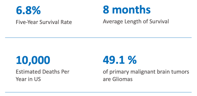
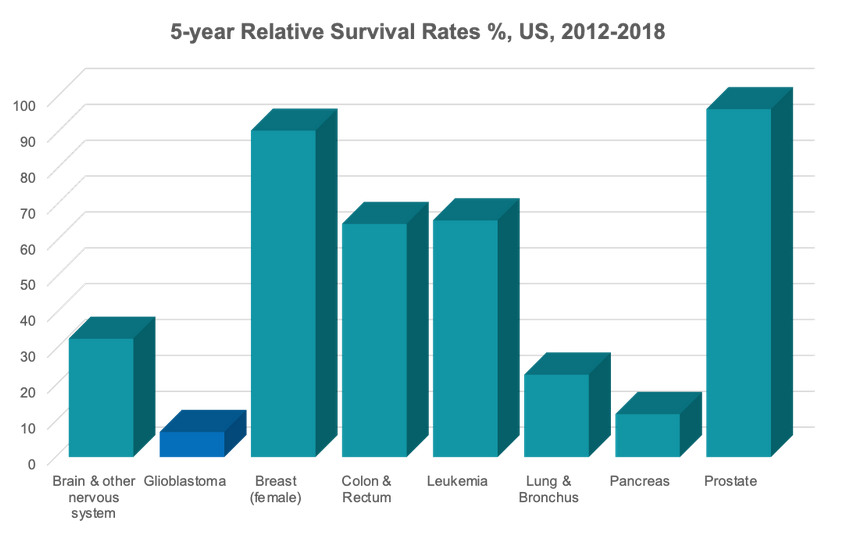
os.chdir(working_dir)

Description

Our team's capstone project focuses on the application of current state-of-the-art (SOTA) computer vision models to 3D MRI volumes of patients diagnosed with Glioblastoma cancer. Glioblastoma (GBM) is a very aggressive form of cancer, and "survival rates and mortality statistics for GMB have been virtually unchanged for decades." Data source: BrainTumor.org

Our motivations include:

1. Advance diagnostic, treatment, and medical research
2. Test novel data science tools on 2D and 3D image data
3. Support exploration applications in the energy industry (image data idea transfer, such as 3D seismic data)

Our objectives are to develop machine learning tools focused on:

1. Automated Brain Tumor Segmentation
2. Biomaker prediction (classification)
3. Brain Tumor detection (classification / anomaly detection)

Data

We are using a data set from the Cancer Imaging Archive for segmentation and classification of brain MRI scans for patients diagnosed to have Glioblastoma-type cancer. The data is hosted here and is collected and made available by the University of Pennsylvania Health System.

Data citation:

Bakas, S., Sako, C., Akbari, H., Bilello, M., Sotiras, A., Shukla, G., Rudie, J. D., Flores Santamaria, N., Fathi Kazerooni, A., Pati, S., Rathore, S., Mamourian, E., Ha, S. M., Parker, W., Doshi, J., Baid, U., Bergman, M., Binder, Z. A., Verma, R., … Davatzikos, C. (2021). Multi-parametric magnetic resonance imaging (mpMRI) scans for de novo Glioblastoma (GBM) patients from the University of Pennsylvania Health System (UPENN-GBM) (Version 2) [Data set]. The Cancer Imaging Archive. https://doi.org/10.7937/TCIA.709X-DN49

Publication citation:

Bakas, S., Sako, C., Akbari, H., Bilello, M., Sotiras, A., Shukla, G., Rudie, J. D., Flores Santamaria, N., Fathi Kazerooni, A., Pati, S., Rathore, S., Mamourian, E., Ha, S. M., Parker, W., Doshi, J., Baid, U., Bergman, M., Binder, Z. A., Verma, R., Lustig, R., Desai, A. S., Bagley, S. J., Mourelatos, Z., Morrissette, J., Watt, C. D., Brem, S., Wolf, R. L., Melhem, E. R., Nasrallah, M. P., Mohan, S., O’Rourke, D. M., Davatzikos, C. (2022). The University of Pennsylvania glioblastoma (UPenn-GBM) cohort: advanced MRI, clinical, genomics, & radiomics. In Scientific Data (Vol. 9, Issue 1). https://doi.org/10.1038/s41597-022-01560-7

TCIA citation:

Clark, K., Vendt, B., Smith, K., Freymann, J., Kirby, J., Koppel, P., Moore, S., Phillips, S., Maffitt, D., Pringle, M., Tarbox, L., & Prior, F. (2013). The Cancer Imaging Archive (TCIA): Maintaining and Operating a Public Information Repository. Journal of Digital Imaging, 26(6), 1045–1057. https://doi.org/10.1007/s10278-013-9622-7

The data set is licensed under CC BY 4.0

This data set includes:

1. 3D mpMRI Images
   • T1, T2, T1-GD, and T2-Flair attribute volumes (~630 patients of 1-5+ GB each, 800,000+ images)
   • DICOM and NIFTI format
     • NIFTI images are skull-stripped and registered
   • Cancerous and non-cancerous instances
   • Additional dataset of MRI images from normal, healthy patients (600 images with T1, T2, and PD-weighted attributes)
2. Brain Tumor annotations
   • de novo Glioblastoma tumors
   • 3D volumes for multiple patients
3. Histopathology slides
   • RGB images
4. Clinical data
   • survival dates after surgery
   • MGMT (Unmethylated, Indeterminate, Methylated)
   • IDH1
   • Demographics

Data Science Pipeline

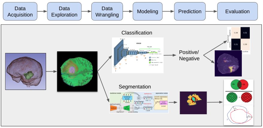
A high level summary of our data science pipline is as follows:

1. Data Acquisition
2. Data Exploration
3. Data Wrangling
4. Modeling
5. Prediction (Inference)
6. Evaluation

Through data acquistion, exploration, and wrangling, we convert 3D MRI volumes into 2D RGB images for use in our models.

For classification, we use a convolutional neural network called VGG19 to predict if an image contains a tumor.

For segmentation, we use a vision transformer called Maskformer to predict the tumor segments within a 2D image.

Following the modeling tasks, we quantitatively evaluate the prediction results.