Check out the presentation slides for this work here at Neural Uncertainty for Differential Emotion Perception
Understanding the Human Brain's working have always fascinated me. The way we learn from things, the way we abstract an idea in our brain, the way we percieve and think of things around us is all related to the highly evolved organ- The Human Brain. From the ancient times, endeavours were made by philosophers to understand the functioning of brain and how it abstracts concepts and feelings. In the past of these modern times, scientists tried several methods, techniques, experiments and theory to explain the complex brain functions and even more complex the representation of emotions in human brain. That is exactly what we try to deal with here.
Understanding the dynamics of our affective experiences has been one of the hardest problems in the field of neuroscience owing to the complexity of the phenomenon. Prevalent theories have mainly tried to characterize emotions using two dimensions of Arousal and Valence. However, empirical works have shown that these are insufficient in explaining real-life complexity and dynamicity of our affective experiences. In this domain, an unresolved question that still exists is how these emotional experiences change with age. Basing our work on a previous study which showed uncertainty to be a central parameter in mediating affective dynamics, we tried to explain the differential emotional experience in older individuals from a representational and computational level, using unsupervised approaches and sophisticated neural network models.
In the past, emotions are understood as a combination of two measures of Valence and Arousal. Hence, analysis or work on emotions previously meant collecting data on these two variables for each individual. But as per the recent work by Majumdar et. al., it proposes that uncertainty plays an important role in explaining the emotional dynamics. Hence, the objective of our study is to explore this hypothesis as well as trying to come up with a quantification of uncertainty.
Another major objective of the study is to compare the emotional response between young and old subjects based on the significant difference in uncertainty processing. So, we hypothesize that the lack of uncertainty representation might be the reason of difference in emotions exhibited by young and old subjects. Hence, another goal of our study is to find a sufficient method for uncertainty representation.
Although both the above goals might be similar, the first one deals with quantitative analysis of uncertainty whereas the second one maybe a visual representation.
In our study we analyzed the behavioral data of participants on a Facial recognition task where they were presented with different faces portraying either of the
For the neural analyses we examined the neuroimaging responses of participants to a tailored version (
A total of
After preprocessing the fMRI (functional Magnetic Resonance Imaging) data, we extracted the BOLD (Blood Oxygen Level Dependent) timeseries for all participants for this movie watching task. The first
The final pre-processed data of the
For the representational level we wanted to explore the low dimensional manifolds for representation of uncertainty in Young and Old using few data driven analyses. We also carry out computational level of analysis later to capture uncertainty related information.
Dimension Reduction is a well-known technique for feature extraction and data-visualization of high-dimensional data. In our case, we want to extract low-dimensional signature or pattern of the averaged data
- Principle Component Analysis(PCA)
- t-Distributed Stochastic Neighbor Embedding (t-SNE)
- Potential of Heat-diffusion for Affinity-based Trajectory Embedding(PHATE)
- Temporal Potential of Heat-diffusion for Affinity-based Trajectory Embedding(TPHATE)
The principal components of a collection of points in a real coordinate space are a sequence of
The PCA algorithm works by finding the eigenvalues and eigenvectors of the data matrix using Singular Value Decomposition(SVD) and then ordering the eigenvectors in descending order based on the eigenvalues and then picking up first few eigenvectors as the basis and reconstructing the data back by using these new loading vectors. Eigenvalues give the idea about the strength or variance explained.
In our case we applied PCA on the matrix
PCA captures the overall global relationship in the data at the cost of shattering local information, like proximity of two points or similar characteristics.
t-SNE is a statistical method for visualizing high-dimensional data by giving each datapoint a location in a two or three-dimensional map. It is a nonlinear dimensionality reduction technique well-suited for embedding high-dimensional data for visualization in a low-dimensional space of two or three dimensions. Specifically, it models each high-dimensional object by a two- or three-dimensional point in such a way that similar objects are modeled by nearby points and dissimilar objects are modeled by distant points with high probability.
The t-SNE algorithm comprises two main stages. First, t-SNE constructs a probability distribution over pairs of high-dimensional objects in such a way that similar objects are assigned a higher probability while dissimilar points are assigned a lower probability. Second, t-SNE defines a similar probability distribution over the points in the low-dimensional map, and it minimizes the Kullback–Leibler divergence (KL divergence) between the two distributions with respect to the locations of the points in the map.
In our case we applied PCA on the matrix
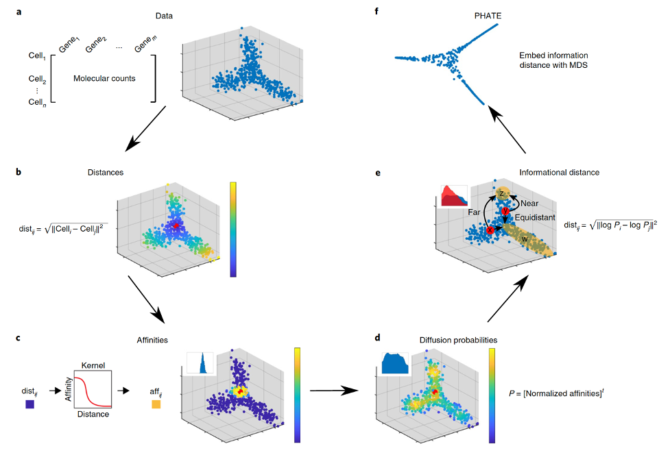
PHATE provides a denoised, two or three-dimensional visualization of the complete branching trajectory structure in high-dimensional data. It uses heat-diffusion processes, which naturally denoise the data, to compute data point affinities. Then, PHATE creates a diffusion-potential geometry by free-energy potentials of these processes. This geometry captures high-dimensional trajectory structures, while enabling a natural embedding of the intrinsic data geometry. This embedding accurately visualizes trajectories and data distances, without requiring strict assumptions typically used by path-finding and tree-fitting algorithms, which have recently been used for pseudotime orderings or tree-renderings of high dimensional data with hierarchy.
Given a dataset of voxel time-series data,
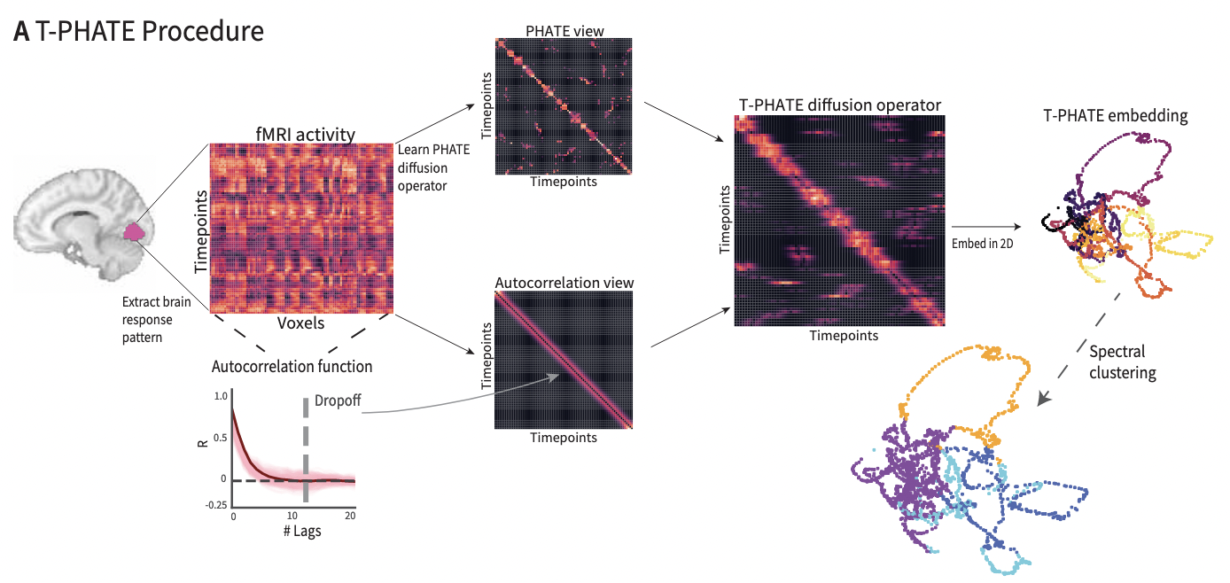
TPHATE is a modified PHATE algorithm which is able to capture the temporal aspect of the data. The algorithm works the same as original PHATE except for the temporal component infused in the diffusion matrix using the auto-covariance function in a Temporal Affinity Matrix, which is explained below.
TPHATE as a variant of PHATE that uses a dual-view diffusion operator to embed timeseries data in a low-dimensional space. The first view,
Sequence Modeling is the technique of training models on data that has a temporal component associated with it to predict the next value/state. Realizing that our data matrix
- Long Short-Term Memory Neural Network(LSTM)
LSTMs are better than Recurrent Neural Networks(RNN) at carrying information from past time steps to farther time steps ahead and improves gradient update values preventing issues like vanishing or exploding gradients which is an issue with RNNs.
LSTM unit has a memory cell and three gates: input gate, output gate and forget gate. Intuitively, at time step
Mathematically, the states of LSTM are updated as follows:
For prediction at each time step we pass the hidden state
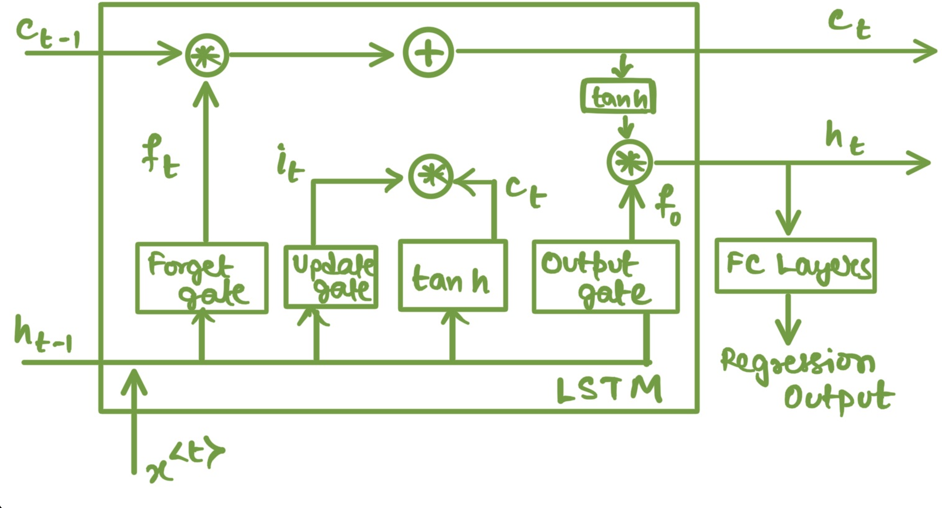 Long Short-Term Memory Cell gates and information flow diargam
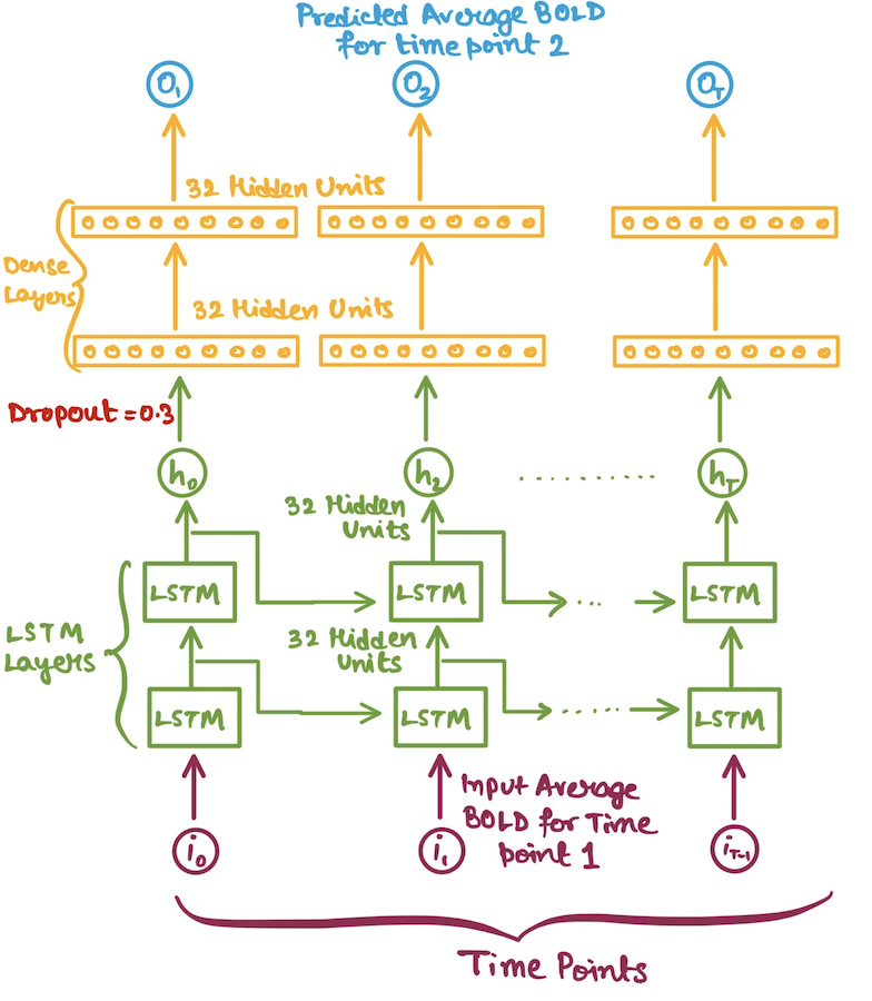
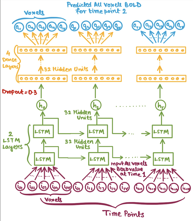
In our case we would be using LSTMs for a regression setup. But the problem arises of how to feed in the inputs to our LSTM model? Since, our data is high-dimensional i.e. the number of voxels per ROI is quite high(atleast
So, we decide on using the following inputs for each subject:
- Average BOLD values(averaged across the voxel BOLDs) for each time point.
- Multivariate BOLD values for each time point(i.e. no reduction number of voxels).
Now, after deciding on the inputs, we have no prior knowledge of what model hyperparameters would suffice or perform the best compared to the others. Hence, we used several different hyperparameter combinations from the following choices:
-
$1, 2, 3$ LSTM Layers -
$8, 16, 32, 64, 128$ Hidden Units -
$1, 2, 3, 4$ Dense Layers -
$0.3$ Dropout Probability
Now, the model is trained using Mini-Batch Gradient Descent. We used Adam Optimizer. We trained the models on each ROI separately for
| Average BOLD LSTM | Multivariate(All) BOLD LSTM |
|---|---|
 |
 |
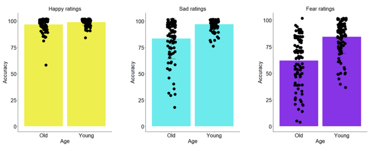
To prove that the older people have differential emotion perception than the Young individuals, we looked into their accuracy for the FER task for the Happy, Sad and Fear emotions. We found that for all three emotions the accuracy differed significantly between the two groups (Happy: Mean Accuracy:
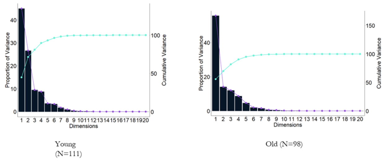
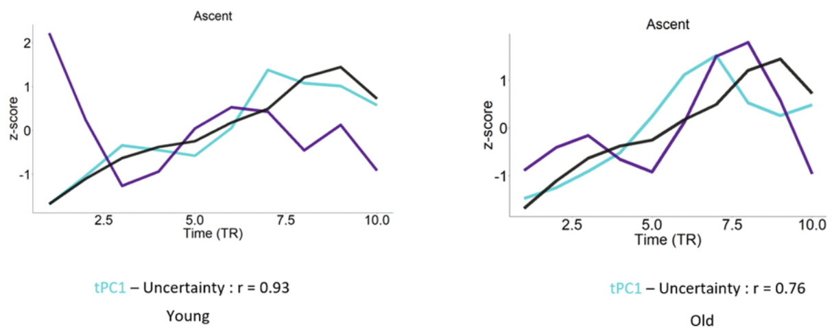
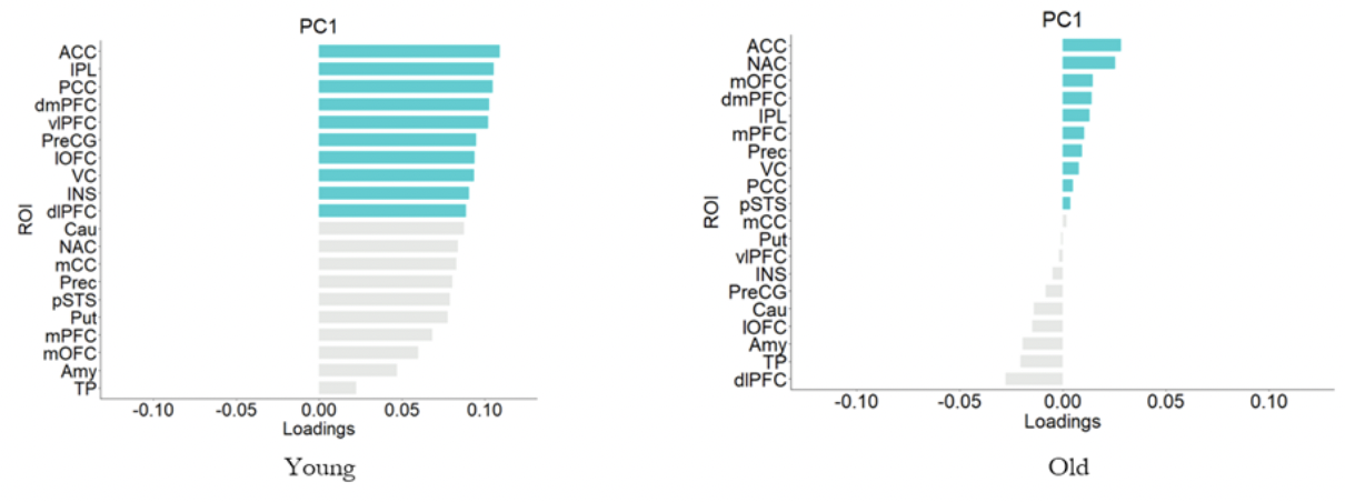
We employed a spatio-temporal PCA on the BOLD time series extracted from
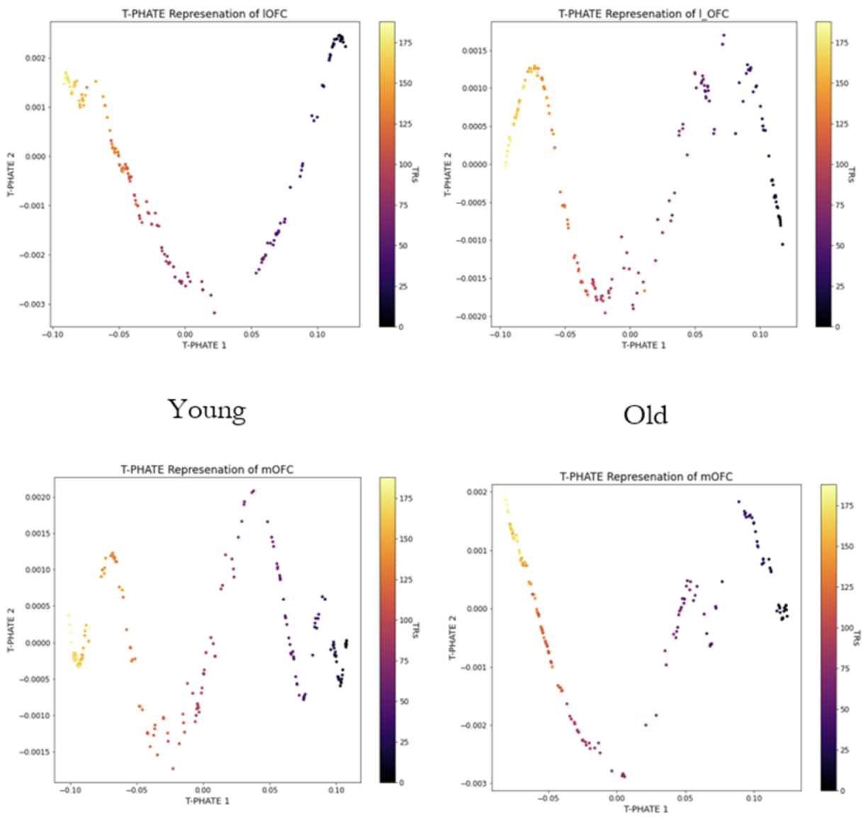
A recent study showed that for complex representation architecture Temporal PHATE can capture both the global and local information of the data thus adding onto our previous result. We wanted to see whether we can find a significant difference in the low dimensional signature of the lateral and medial orbitofrontal cortex by implementing this TPHATE. The motivation for choosing these areas comes from the previous work from this lab.
*TPHATE on the voxel wise BOLD data of the lOFC and mOFC for the Young and the Old*As per the methodology described in the previous section, we after training the models with different sets of hyperparameters and architectures tracked the model performances based on the following criterias:
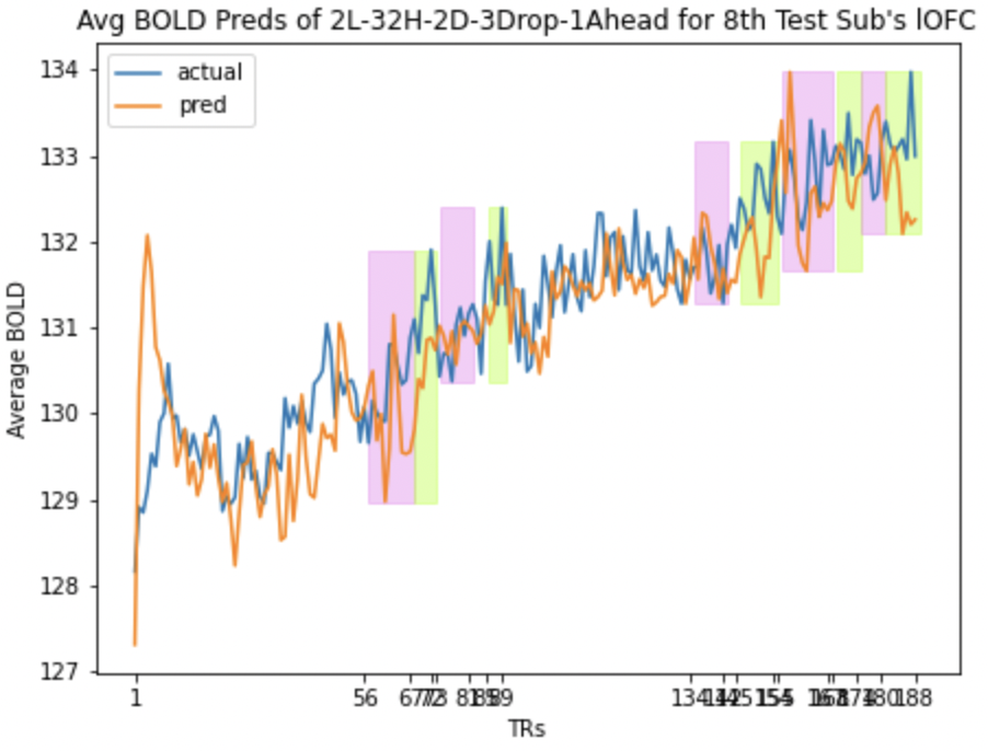
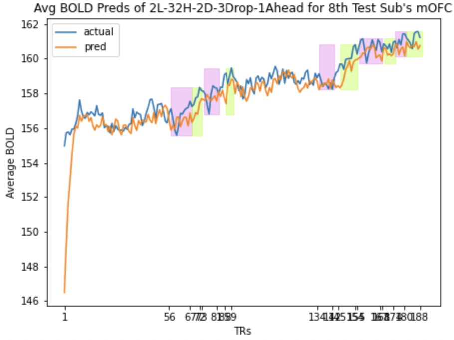
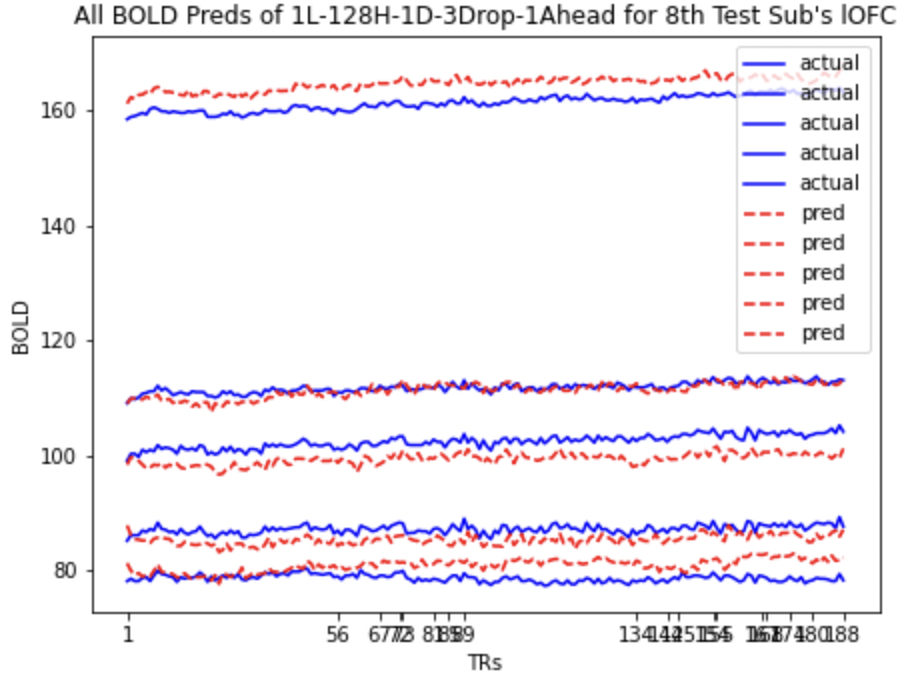
- Correlation between the actual and predicted BOLD signals for the validation subjects.
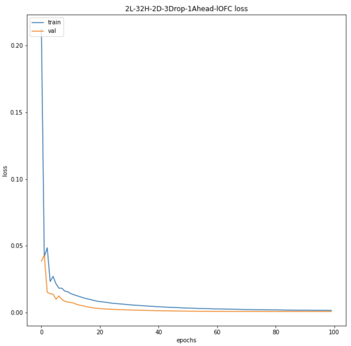
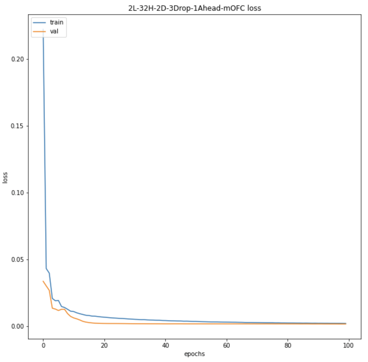
- Scaled training subjects mean squared error loss.
- Scaled validation subjects mean squared error loss.
- Validation subjects mean squared loss.
- Ascent and descent wise actual and predicted BOLD correlation for validation subjects.
We also look at the prediction plots, training loss and validation loss plots to identify any problem with the models.
Here we present the predictions for mOFC and lOFC of the
| lOFC | mOFC |
|---|---|
 Average BOLD LSTM Predictions Average BOLD LSTM Predictions |
 Average BOLD LSTM Predictions Average BOLD LSTM Predictions |
 Average BOLD LSTM Loss Average BOLD LSTM Loss |
 Average BOLD LSTM Loss Average BOLD LSTM Loss |
Here we present the predictions for mOFC and lOFC of the
| lOFC | mOFC |
|---|---|
 All BOLD LSTM Predictions All BOLD LSTM Predictions |
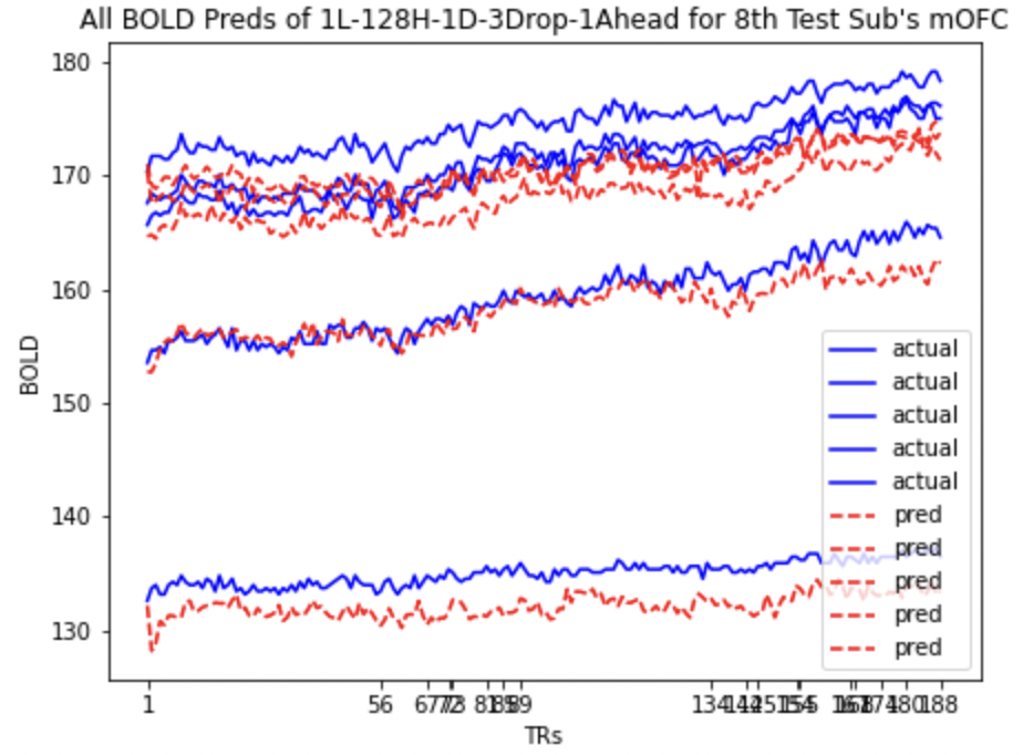 All BOLD LSTM Predictions All BOLD LSTM Predictions |
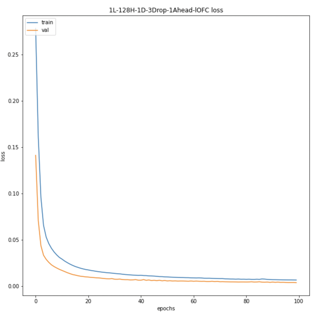 All BOLD LSTM Loss All BOLD LSTM Loss |
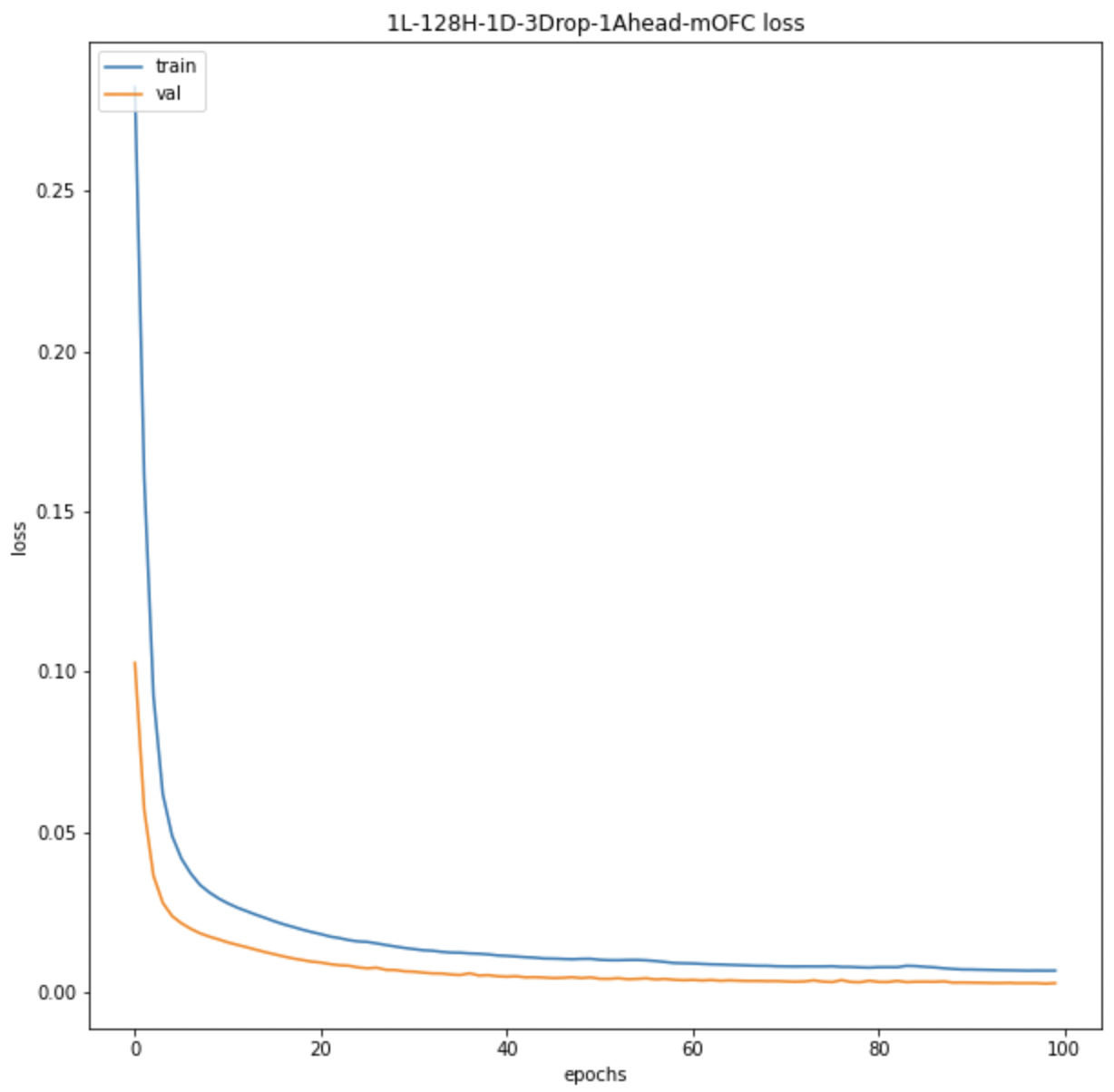 All BOLD LSTM Loss All BOLD LSTM Loss |
By analysing the neuroimaging data using multiple data unsupervised approaches, we observed that the low dimensional representation of the lOFC and mOFC completely shifts from Young to Old. Since lOFC has already been implicated in mediating the Uncertainty in Young this gives us an interesting avenue to look into future. The preliminary LSTM models gave us an few potential branches that we can follow to explore the our main question on estimating how far ahead uncertainty is estimated in Young and Old.
There are a sequence of work lined up following this analysis. Where we will crack down concretely on the computational models and representation extracted from these computational models both quantitative and visual to represent uncertainty.
Some of the upcoming areas which we plan to extend our work to are:
- Using low-dimensional extracted features like TPHATE along with BOLD values of voxels to see if there is significant improvement in the model being able to capture the uncertainty based information.
- Using Masked Attention Based LSTM Model to extract parts of the BOLD time series to which the model pays most attention for BOLD value predictions of the descents.
- The current models are trained on young subjects data, so we will be using the selected model for the old subjects to compare the results and accuracy.
- Coming to the raised question of how far ahead the young subjects are predicting compared to the old subjects we will train the selected model for
$2$ TR,$3$ TR, …, upto$15$ TR ahead prediction and compare the slopes of prediction loss and correlation. - Using Multi-Modality of our data i.e. incorporating Movie frames information along with BOLD values for each ROIs and coming up with a uncertainty map of regions of focus in the movie as well as the ROIs responsible.
- Devise or track other measures for model selection as well as quantify uncertainty based on metrics for similarity and distance between actual and predicted signals.
- Reduced Voxel Dimensionality using unsupervised methods to extract maximum relevant information.
-
Plots: Contains all the Plots generated from the analysis or codes written in the notebooks. It contains subfolders forYOUNGandOLD, with further subfolders ofPCA, etc. corresponding to the class of analysis to which it belongs. -
Models: Contains the trained model weights of various architectures and set of hyperparameters. Named accordingly, wheremodel_weights-1L-128H-1D-3Drop-1Ahead-mOFCmeans the weights for the model with$1$ LSTM Layer,$128$ Hidden Units in the Dense Layers(Except Last Layer which has either$1$ unit for Average BOLD LSTM or Number of Voxels units for All BOLD LSTM) and the LSTM Layers,$1$ Dense Layer,$0.3$ Dropout Probability and it is trained for predicting$1$ TR ahead BOLD values. -
Model-Inference: Contains the outputs such as predicted BOLD values generated by Models and other numerical outputs which are not plots. -
Report: Contains the reports and presentations for intermediate progresses. -
Jupyter Notebooks(.ipynb): Contains the code for the analysis and important values like correlation, MSE loss, etc.
