tensor-network-ahs

This package implements a tensor network based algorithm for simulating Rydberg atom dynamics. It allows to simulate Analog Hamiltonian Simulation programs for problem sizes of hundreds of atoms, which is unaccessible by statevector simulation methods. Matrix Product States (MPS) are used to represent the many-body quantum state.

The core of the tensor network simulation is enabled by iTensor.jl. The input Analog Hamiltonian Simulation (AHS) program can be constructed using Braket.jl interface.

Introduction

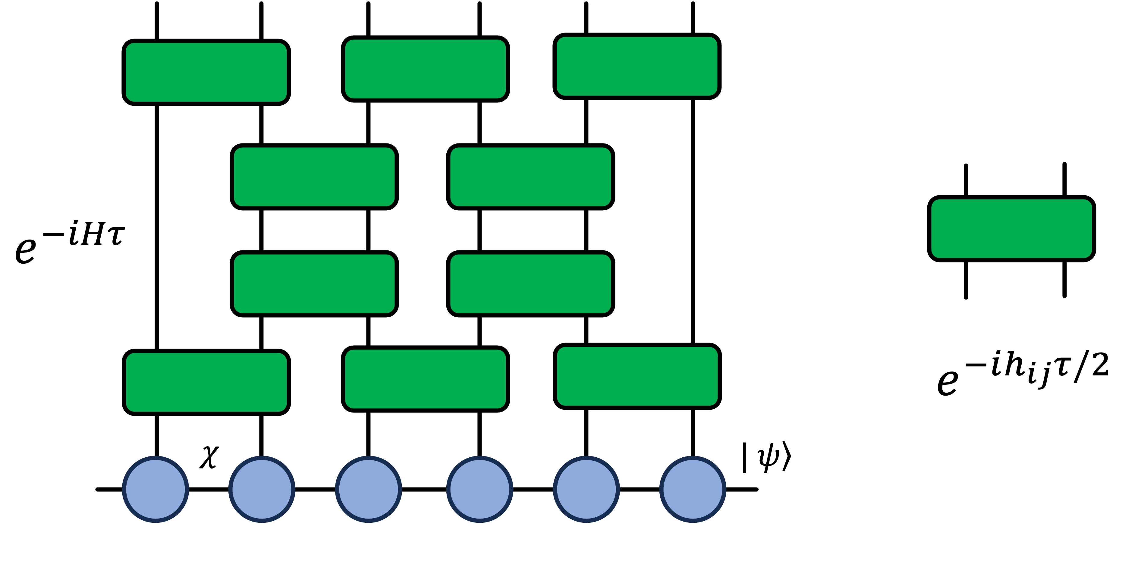
We use Time Evolving Block Decimation (TEBD) algorithm to compute state updates for each time step. After each TEBD step the quantum state is truncated based on the SVD decomposition of the matrix product state. The second order Suzuki-Trotter product formula is used for improved simulation accuracy.

A step of TEBD evolution acting on a matrix product state is pictorially shown below.

Computational cost (for each evolution step): $O(χ^3)$, where $χ$ is the current MPS bond dimension. For the purpose of efficient MPS simulation we perform truncation of the van der Waals terms for distances exceeding a fixed interation-radius (supplied as an input argument).

Getting started

Install Julia to your machine. To install relevant Julia packages cd to the project root and execute

julia --project=. -e 'using Pkg; Pkg.instantiate()'

Running MPS-based simulation

To run the Braket-AHS program saved as a .json file run:

julia src/mps_runner.jl --program-path=<path_to_ahs.json>

In order to generate .json configuration file there are 2 options:

1.A Generate .json using Braket.jl interface provided in srs/ahs_program.jl.

julia src/ahs_program.jl

The output .json file will be saved in examples/ahs_program.json.

1.B Generate .json using Python Braket SDK from the AHS program object:

ahs_ir = ahs_program.to_ir()
json_object = json.loads(ahs_ir.json())
json_string = json.dumps(json_data, indent=4) 
filename = "ahs_program.json"
with open(filename, "w") as json_file:
    json_file.write(json_string)

Example .json config files are provided in examples/ahs_program*.json.

The required input argument is:

--program-path: specifies the path to AHS program .json file (example file is provided examples/ahs_program.json)

The optional arguments are:

--experiment-path: directory where all experiment results are saved (default is examples/experiment_braket).
--interaction-radius: interaction radius [in meters], only interaction between atoms within the interaction radius are taken into account during MPS simulation (van der Waals tail is truncated for Rij>interaction_radius resulting in Vij=0). The default value is interaction-radius=7e-6.
--cutoff: SVD truncation cutoff parameter for each step of TEBD evolution. The default value is cutoff=1e-7.
--shots: number of bitstring samples at final time step. Samples are saved in <experiment_path>/samples.csv. Default value is shots=1000.
--max-bond-dim: maximum MPS bond dimension throughout TEBD evolution. In case if the bond dimension competes with cutoff parameter, the max-bond-dim takes priority - the MPS bond dimension can not grow beyond maximum value.
--tau: Trotter time step [in seconds]. Default value is tau=1e-8 (seconds).
--n-tau-steps: total number of Trotter steps. The total evolution time is tau*n-tau-steps. Default value is n-tau-steps=400, corresponds to total evolution time 4 microseconds.
--C6: Rydberg interaction C6 constant, default value is C6=5.42e-24 (CI units).
--compute-truncation-error: computes MPS truncation error for each time step and saves truncation error evolution in <experiment_path>/error_log.txt. Use with CAUTION, since enabling this option dramatically slows down runtime (requires calculation of exact MPS evolution for each time step).
--compute-correlators: compute <Z_i Z_j> correlators for all pairs of atoms at the end of the evolution.
--compute-energies: compute energies from samples at the end of the evolution.
--generate-plots: generate plots after experiment is finished

MPS-results

Output files from MPS simulaiton are stored in <experiment_path>:

ahs_program.json: copy of the AHS program .json file.
atom_coordinates.csv: Atom coordinates in 2D plane [in meters].
mps_density.csv: evolution of <n_i>(t) for each atom as a function of time.
mps_samples.csv: bitstring samples from MPS at t=T.
correlator_zz.csv: ZZ correlation function at final time t=T: <Sz_i Sz_j>.
energies.csv: final energies corresponding to the MPS samples at t=T.
summary.txt: summary file with the experiment information (runtime, input args, etc.)

Visualization

To run visualization script run:

julia src/plotter.jl <path_to_experiment_results>

It will generate plots from the .csv files saved in <path_to_experiment_results>.

Roshan-Thomas/BraketAHS.jl