Referenced paper : Text Classification Algorithms: A Survey
- Introduction
- Text and Document Feature Extraction
- Dimensionality Reduction
- Text Classification Techniques
- Rocchio classification
- Boosting and Bagging
- Naive Bayes Classifier
- K-nearest Neighbor
- Support Vector Machine (SVM)
- Decision Tree
- Random Forest
- Conditional Random Field (CRF)
- Deep Learning
- Comparison Text Classification Algorithms
- Evaluation
- Text and Document Datasets
- Text Classification Applications
- Text Classification Support
- Citations:
Text feature extraction and pre-processing for classification algorithms are very significant. In this section, we start to talk about text cleaning since most of documents contain a lot of noise. In this part, we discuss two primary methods of text feature extractions- word embedding and weighted word.
In Natural Language Processing (NLP), most of the text and documents contain many words that are redundant for text classification, such as stopwords, miss-spellings, slangs, and etc. In this section, we briefly explain some techniques and methods for text cleaning and pre-processing text documents. In many algorithms like statistical and probabilistic learning methods, noise and unnecessary features can negatively affect the overall perfomance. So, elimination of these features are extremely important.
Tokenization is the process of breaking down a stream of text into words, phrases, symbols, or any other meaningful elements called tokens. The main goal of this step is to extract individual words in a sentence. Along with text classifcation, in text mining, it is necessay to incorporate a parser in the pipeline which performs the tokenization of the documents; for example:
sentence:
After sleeping for four hours, he decided to sleep for another four
In this case, the tokens are as follows:
{'After', 'sleeping', 'for', 'four', 'hours', 'he', 'decided', 'to', 'sleep', 'for', 'another', 'four'}
Here is python code for Tokenization:
from nltk.tokenize import word_tokenize
text = "After sleeping for four hours, he decided to sleep for another four"
tokens = word_tokenize(text)
print(tokens)Text and document classification over social media, such as Twitter, Facebook, and so on is usually affected by the noisy nature (abbreviations, irregular forms) of the text corpuses.
Here is an exmple from geeksforgeeks
from nltk.corpus import stopwords
from nltk.tokenize import word_tokenize

example_sent = "This is a sample sentence, showing off the stop words filtration."

stop_words = set(stopwords.words('english'))

word_tokens = word_tokenize(example_sent)

filtered_sentence = [w for w in word_tokens if not w in stop_words]

filtered_sentence = []

for w in word_tokens:
    if w not in stop_words:
        filtered_sentence.append(w)

print(word_tokens)
print(filtered_sentence)
Output:
['This', 'is', 'a', 'sample', 'sentence', ',', 'showing',
'off', 'the', 'stop', 'words', 'filtration', '.']
['This', 'sample', 'sentence', ',', 'showing', 'stop',
'words', 'filtration', '.']Sentences can contain a mixture of uppercase and lower case letters. Multiple sentences make up a text document. To reduce the problem space, the most common approach is to reduce everything to lower case. This brings all words in a document in same space, but it often changes the meaning of some words, such as "US" to "us" where first one represents the United States of America and second one is a pronoun. To solve this, slang and abbreviation converters can be applied.
text = "The United States of America (USA) or America, is a federal republic composed of 50 states"
print(text)
print(text.lower())
Output:
"The United States of America (USA) or America, is a federal republic composed of 50 states"
"the united states of america (usa) or america, is a federal republic composed of 50 states"
Slangs and abbreviations can cause problems while executing the pre-processing steps. An abbreviation is a shortened form of a word, such as SVM stand for Support Vector Machine. Slang is a version of language that depicts informal conversation or text that has different meaning, such as "lost the plot", it essentially means that 'they've gone mad'. Common method to deal with these words is converting them to formal language.
Another issue of text cleaning as a pre-processing step is noise removal. Text documents generally contains characters like punctuations or special characters and they are not necessary for text mining or classification purposes. Although punctuation is critical to understand the meaning of the sentence, but it can affect the classification algorithms negatively.
Here is simple code to remove standard noise from text:
def text_cleaner(text):
    rules = [
        {r'>\s+': u'>'},  # remove spaces after a tag opens or closes
        {r'\s+': u' '},  # replace consecutive spaces
        {r'\s*<br\s*/?>\s*': u'\n'},  # newline after a <br>
        {r'</(div)\s*>\s*': u'\n'},  # newline after </p> and </div> and <h1/>...
        {r'</(p|h\d)\s*>\s*': u'\n\n'},  # newline after </p> and </div> and <h1/>...
        {r'<head>.*<\s*(/head|body)[^>]*>': u''},  # remove <head> to </head>
        {r'<a\s+href="([^"]+)"[^>]*>.*</a>': r'\1'},  # show links instead of texts
        {r'[ \t]*<[^<]*?/?>': u''},  # remove remaining tags
        {r'^\s+': u''}  # remove spaces at the beginning
    ]
    for rule in rules:
    for (k, v) in rule.items():
        regex = re.compile(k)
        text = regex.sub(v, text)
    text = text.rstrip()
return text.lower()An optional part of the pre-processing step is correcting the misspelled words. Different techniques, such as hashing-based and context-sensitive spelling correction techniques, or spelling correction using trie and damerau-levenshtein distance bigram have been introduced to tackle this issue.
from autocorrect import spell

print spell('caaaar')
print spell(u'mussage')
print spell(u'survice')
print spell(u'hte')
Result:
caesar
message
service
the
Text Stemming is modifying a word to obtain its variants using different linguistic processeses like affixation (addition of affixes). For example, the stem of the word "studying" is "study", to which -ing.
Here is an example of Stemming from NLTK
from nltk.stem import PorterStemmer
from nltk.tokenize import sent_tokenize, word_tokenize

ps = PorterStemmer()

example_words = ["python","pythoner","pythoning","pythoned","pythonly"]

for w in example_words:
print(ps.stem(w))
Result:
python
python
python
python
pythonli
Text lemmatization is the process of eliminating redundant prefix or suffix of a word and extract the base word (lemma).
from nltk.stem import WordNetLemmatizer

lemmatizer = WordNetLemmatizer()

print(lemmatizer.lemmatize("cats"))Different word embedding procedures have been proposed to translate these unigrams into consummable input for machine learning algorithms. A very simple way to perform such embedding is term-frequency~(TF) where each word will be mapped to a number corresponding to the number of occurrence of that word in the whole corpora. The other term frequency functions have been also used that represent word-frequency as Boolean or logarithmically scaled number. Here, each document will be converted to a vector of same length containing the frequency of the words in that document. Although such approach may seem very intuitive but it suffers from the fact that particular words that are used very commonly in language literature might dominate this sort of word representations.
Original from https://code.google.com/p/word2vec/
I’ve copied it to a github project so that I can apply and track community patches (starting with capability for Mac OS X compilation).
- makefile and some source has been modified for Mac OS X compilation See https://code.google.com/p/word2vec/issues/detail?id=1#c5
- memory patch for word2vec has been applied See https://code.google.com/p/word2vec/issues/detail?id=2
- Project file layout altered
There seems to be a segfault in the compute-accuracy utility.
To get started:
cd scripts && ./demo-word.sh
Original README text follows:
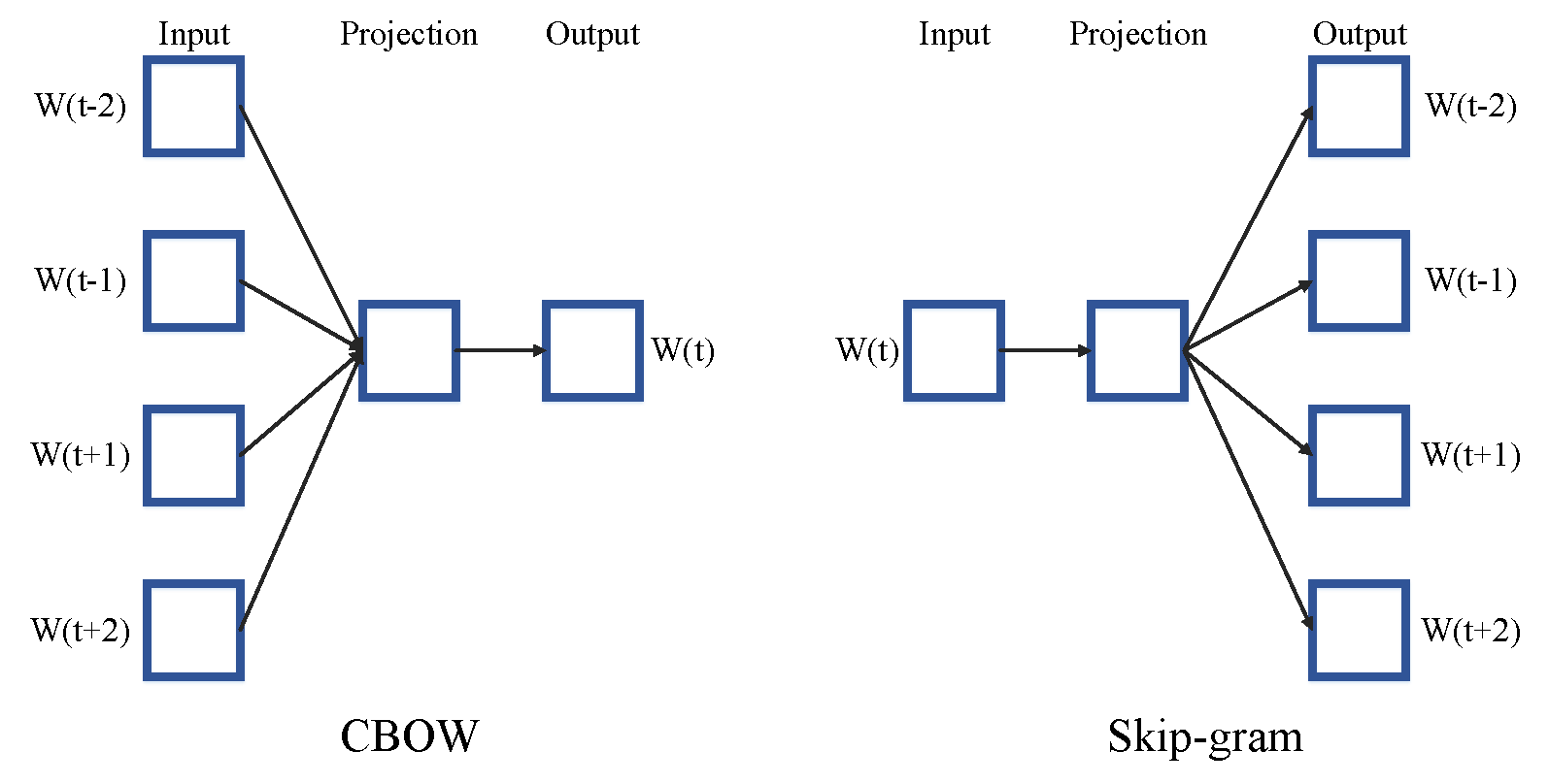
This tool provides an efficient implementation of the continuous bag-of-words and skip-gram architectures for computing vector representations of words. These representations can be subsequently used in many natural language processing applications and for further research purposes.
this code provides an implementation of the Continuous Bag-of-Words (CBOW) and the Skip-gram model (SG), as well as several demo scripts.
Given a text corpus, the word2vec tool learns a vector for every word in the vocabulary using the Continuous Bag-of-Words or the Skip-Gram neural network architectures. The user should specify the following: - desired vector dimensionality (size of the context window for either the Skip-Gram or the Continuous Bag-of-Words model), training algorithm (hierarchical softmax and / or negative sampling), threshold for downsampling the frequent words, number of threads to use, format of the output word vector file (text or binary).
Usually, other hyper-parameters, such as the learning rate do not need to be tuned for different training sets.
The script demo-word.sh downloads a small (100MB) text corpus from the web, and trains a small word vector model. After the training is finished, users can interactively explore the similarity of the words.
More information about the scripts is provided at https://code.google.com/p/word2vec/
An implementation of the GloVe model for learning word representations is provided, and describe how to download web-dataset vectors or train your own. See the project page or the paper for more information on glove vectors.
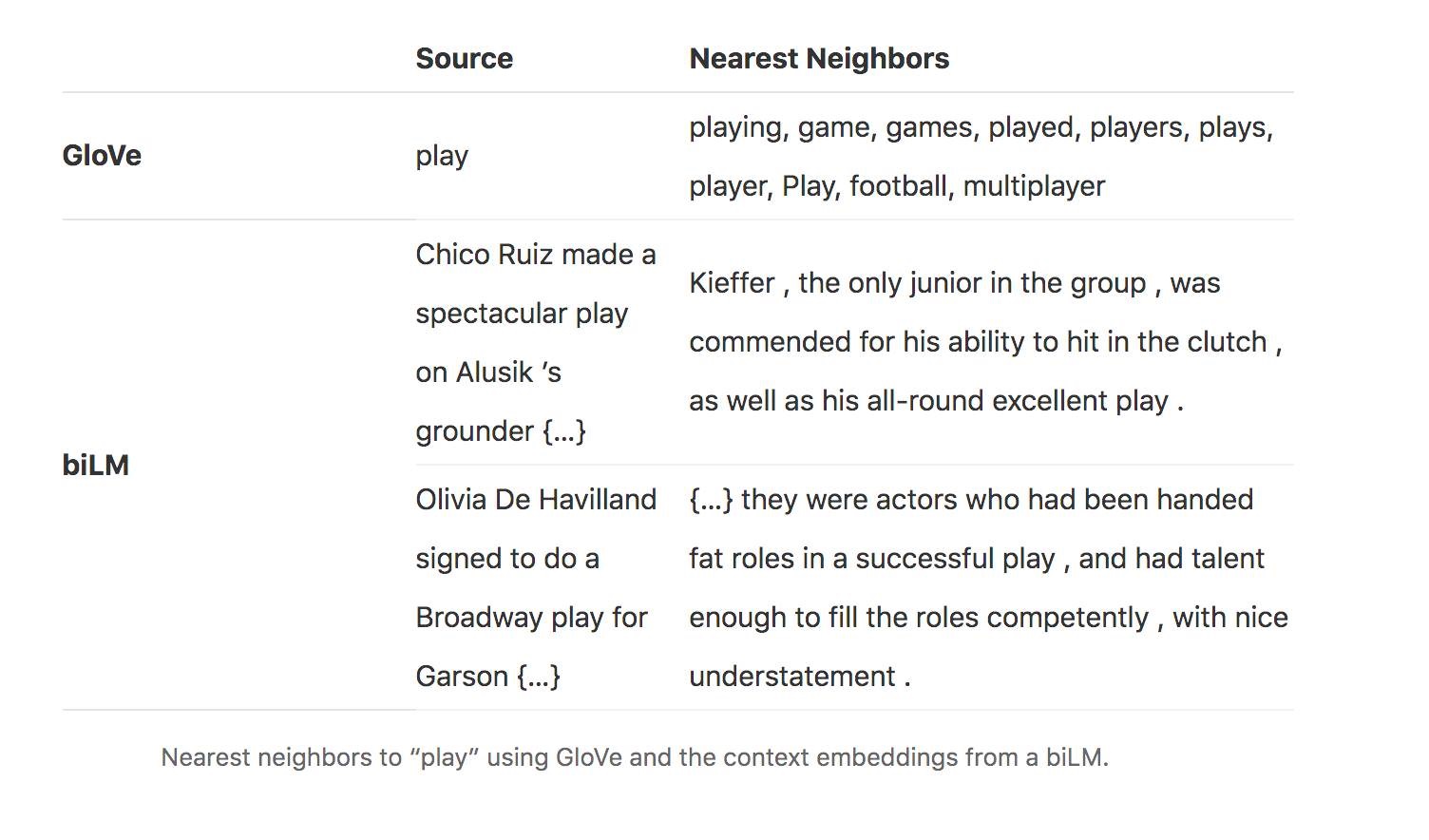
ELMo is a deep contextualized word representation that models both (1) complex characteristics of word use (e.g., syntax and semantics), and (2) how these uses vary across linguistic contexts (i.e., to model polysemy). These word vectors are learned functions of the internal states of a deep bidirectional language model (biLM), which is pre-trained on a large text corpus. They can be easily added to existing models and significantly improve the state of the art across a broad range of challenging NLP problems, including question answering, textual entailment and sentiment analysis.
ELMo representations are:
- Contextual: The representation for each word depends on the entire context in which it is used.
- Deep: The word representations combine all layers of a deep pre-trained neural network.
- Character based: ELMo representations are purely character based, allowing the network to use morphological clues to form robust representations for out-of-vocabulary tokens unseen in training.
Tensorflow implementation
Tensorflow implementation of the pretrained biLM used to compute ELMo representations from "Deep contextualized word representations".
This repository supports both training biLMs and using pre-trained models for prediction.
We also have a pytorch implementation available in AllenNLP.
You may also find it easier to use the version provided in Tensorflow Hub if you just like to make predictions.
pre-trained models:
We have got several pre-trained English language biLMs available for use. Each model is specified with two separate files, a JSON formatted "options" file with hyperparameters and a hdf5 formatted file with the model weights. Links to the pre-trained models are available here.
There are three ways to integrate ELMo representations into a downstream task, depending on your use case.
- Compute representations on the fly from raw text using character input. This is the most general method and will handle any input text. It is also the most computationally expensive.
- Precompute and cache the context independent token representations, then compute context dependent representations using the biLSTMs for input data. This method is less computationally expensive then #1, but is only applicable with a fixed, prescribed vocabulary.
- Precompute the representations for your entire dataset and save to a file.
We have used all of these methods in the past for various use cases. #1 is necessary for evaluating at test time on unseen data (e.g. public SQuAD leaderboard). #2 is a good compromise for large datasets where the size of the file in is unfeasible (SNLI, SQuAD). #3 is a good choice for smaller datasets or in cases where you'd like to use ELMo in other frameworks.
In all cases, the process roughly follows the same steps. First, create a Batcher (or TokenBatcher for #2) to translate tokenized strings to numpy arrays of character (or token) ids. Then, load the pretrained ELMo model (class BidirectionalLanguageModel). Finally, for steps #1 and #2 use weight_layers to compute the final ELMo representations. For #3, use BidirectionalLanguageModel to write all the intermediate layers to a file.
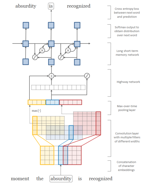
Architecture of the language model applied to an example sentence [Reference: arXiv paper].
fastText is a library for efficient learning of word representations and sentence classification.
Github: facebookresearch/fastText
Models
- Recent state-of-the-art English word vectors.
- Word vectors for 157 languages trained on Wikipedia and Crawl.
- Models for language identification and various supervised tasks.
Supplementary data :
- The preprocessed YFCC100M data .
FAQ
You can find answers to frequently asked questions on Their project website.
Cheatsheet
Also a cheatsheet is provided full of useful one-liners.
Term frequency is Bag of words that is one of the simplest techniques of text feature extraction. This method is based on counting number of the words in each document and assign it to feature space.
The mathematical representation of weight of a term in a document by Tf-idf is given:
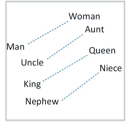
Where N is number of documents and df(t) is the number of documents containing the term t in the corpus. The first part would improve recall and the later would improve the precision of the word embedding. Although tf-idf tries to overcome the problem of common terms in document, it still suffers from some other descriptive limitations. Namely, tf-idf cannot account for the similarity between words in the document since each word is presented as an index. In the recent years, with development of more complex models, such as neural nets, new methods has been presented that can incorporate concepts, such as similarity of words and part of speech tagging. This work uses, word2vec and Glove, two of the most common methods that have been successfully used for deep learning techniques.
from sklearn.feature_extraction.text import TfidfVectorizer
def loadData(X_train, X_test,MAX_NB_WORDS=75000):
    vectorizer_x = TfidfVectorizer(max_features=MAX_NB_WORDS)
    X_train = vectorizer_x.fit_transform(X_train).toarray()
    X_test = vectorizer_x.transform(X_test).toarray()
    print("tf-idf with",str(np.array(X_train).shape[1]),"features")
return (X_train,X_test)| Model | Advantages | Limitation |
| Weighted Words |
|
|
| TF-IDF |
|
|
| Word2Vec |
|
|
| GloVe (Pre-Trained) |
|
|
| GloVe (Trained) |
|
|
| FastText |
|
|
| Contextualized Word Representations |
|
|
Principle component analysis~(PCA) is the most popular technique in multivariate analysis and dimensionality reduction. PCA is a method to identify a subspace in which the data approximately lies. This means finding new variables that are uncorrelated and maximizing the variance to preserve as much variability as possible.
Example of PCA on text dataset (20newsgroups) from tf-idf with 75000 features to 2000 components:
from sklearn.feature_extraction.text import TfidfVectorizer
import numpy as np

def TFIDF(X_train, X_test, MAX_NB_WORDS=75000):
    vectorizer_x = TfidfVectorizer(max_features=MAX_NB_WORDS)
    X_train = vectorizer_x.fit_transform(X_train).toarray()
    X_test = vectorizer_x.transform(X_test).toarray()
    print("tf-idf with", str(np.array(X_train).shape[1]), "features")
    return (X_train, X_test)


from sklearn.datasets import fetch_20newsgroups

newsgroups_train = fetch_20newsgroups(subset='train')
newsgroups_test = fetch_20newsgroups(subset='test')
X_train = newsgroups_train.data
X_test = newsgroups_test.data
y_train = newsgroups_train.target
y_test = newsgroups_test.target

X_train,X_test = TFIDF(X_train,X_test)

from sklearn.decomposition import PCA
pca = PCA(n_components=2000)
X_train_new = pca.fit_transform(X_train)
X_test_new = pca.transform(X_test)

print("train with old features: ",np.array(X_train).shape)
print("train with new features:" ,np.array(X_train_new).shape)

print("test with old features: ",np.array(X_test).shape)
print("test with new features:" ,np.array(X_test_new).shape)
output:
tf-idf with 75000 features
train with old features:  (11314, 75000)
train with new features: (11314, 2000)
test with old features:  (7532, 75000)
test with new features: (7532, 2000)
Linear Discriminant Analysis (LDA) is another commonly used technique for data classification and dimensionality reduction. LDA is particularly helpful where the within-class frequencies are unequal and their performances have been evaluated on randomly generated test data. Class-dependent and class-independent transformation are two approaches in LDA where the ratio of between-class-variance to within-class-variance and the ratio of the overall-variance to within-class-variance are used respectively.
from sklearn.feature_extraction.text import TfidfVectorizer
import numpy as np
from sklearn.discriminant_analysis import LinearDiscriminantAnalysis


def TFIDF(X_train, X_test, MAX_NB_WORDS=75000):
    vectorizer_x = TfidfVectorizer(max_features=MAX_NB_WORDS)
    X_train = vectorizer_x.fit_transform(X_train).toarray()
    X_test = vectorizer_x.transform(X_test).toarray()
    print("tf-idf with", str(np.array(X_train).shape[1]), "features")
    return (X_train, X_test)


from sklearn.datasets import fetch_20newsgroups

newsgroups_train = fetch_20newsgroups(subset='train')
newsgroups_test = fetch_20newsgroups(subset='test')
X_train = newsgroups_train.data
X_test = newsgroups_test.data
y_train = newsgroups_train.target
y_test = newsgroups_test.target

X_train,X_test = TFIDF(X_train,X_test)


LDA = LinearDiscriminantAnalysis(n_components=15)
X_train_new = LDA.fit(X_train,y_train)
X_train_new =  LDA.transform(X_train)
X_test_new = LDA.transform(X_test)

print("train with old features: ",np.array(X_train).shape)
print("train with new features:" ,np.array(X_train_new).shape)

print("test with old features: ",np.array(X_test).shape)
print("test with new features:" ,np.array(X_test_new).shape)
output:
tf-idf with 75000 features
train with old features:  (11314, 75000)
train with new features: (11314, 15)
test with old features:  (7532, 75000)
test with new features: (7532, 15)
from sklearn.feature_extraction.text import TfidfVectorizer
import numpy as np
from sklearn.decomposition import NMF


def TFIDF(X_train, X_test, MAX_NB_WORDS=75000):
    vectorizer_x = TfidfVectorizer(max_features=MAX_NB_WORDS)
    X_train = vectorizer_x.fit_transform(X_train).toarray()
    X_test = vectorizer_x.transform(X_test).toarray()
    print("tf-idf with", str(np.array(X_train).shape[1]), "features")
    return (X_train, X_test)


from sklearn.datasets import fetch_20newsgroups

newsgroups_train = fetch_20newsgroups(subset='train')
newsgroups_test = fetch_20newsgroups(subset='test')
X_train = newsgroups_train.data
X_test = newsgroups_test.data
y_train = newsgroups_train.target
y_test = newsgroups_test.target

X_train,X_test = TFIDF(X_train,X_test)


NMF_ = NMF(n_components=2000)
X_train_new = NMF_.fit(X_train)
X_train_new =  NMF_.transform(X_train)
X_test_new = NMF_.transform(X_test)

print("train with old features: ",np.array(X_train).shape)
print("train with new features:" ,np.array(X_train_new).shape)

print("test with old features: ",np.array(X_test).shape)
print("test with new features:" ,np.array(X_test_new))
output:
tf-idf with 75000 features
train with old features:  (11314, 75000)
train with new features: (11314, 2000)
test with old features:  (7532, 75000)
test with new features: (7532, 2000)
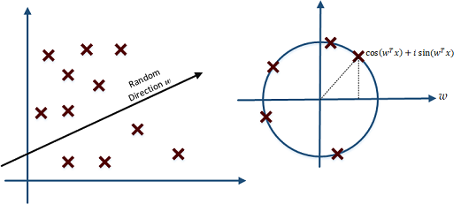
Random projection or random feature is a dimensionality reduction technique mostly used for very large volume dataset or very high dimensional feature space. Text and document, especially with weighted feature extraction, can contain a huge number of underlying features. Many researchers addressed Random Projection for text data for text mining, text classification and/or dimensionality reduction. We start to review some random projection techniques.
from sklearn.feature_extraction.text import TfidfVectorizer
import numpy as np

def TFIDF(X_train, X_test, MAX_NB_WORDS=75000):
    vectorizer_x = TfidfVectorizer(max_features=MAX_NB_WORDS)
    X_train = vectorizer_x.fit_transform(X_train).toarray()
    X_test = vectorizer_x.transform(X_test).toarray()
    print("tf-idf with", str(np.array(X_train).shape[1]), "features")
    return (X_train, X_test)


from sklearn.datasets import fetch_20newsgroups

newsgroups_train = fetch_20newsgroups(subset='train')
newsgroups_test = fetch_20newsgroups(subset='test')
X_train = newsgroups_train.data
X_test = newsgroups_test.data
y_train = newsgroups_train.target
y_test = newsgroups_test.target

X_train,X_test = TFIDF(X_train,X_test)

from sklearn import random_projection

RandomProjection = random_projection.GaussianRandomProjection(n_components=2000)
X_train_new = RandomProjection.fit_transform(X_train)
X_test_new = RandomProjection.transform(X_test)

print("train with old features: ",np.array(X_train).shape)
print("train with new features:" ,np.array(X_train_new).shape)

print("test with old features: ",np.array(X_test).shape)
print("test with new features:" ,np.array(X_test_new).shape)
output:
tf-idf with 75000 features
train with old features:  (11314, 75000)
train with new features: (11314, 2000)
test with old features:  (7532, 75000)
test with new features: (7532, 2000)
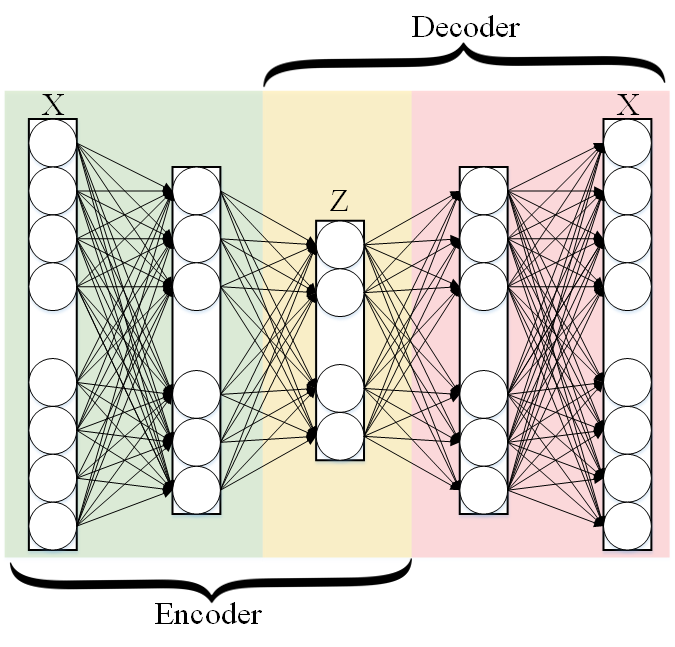
Autoencoder is a neural network technique that is trained to attempt to map its input to its output. The autoencoder as dimensional reduction methods have achieved great success via the powerful reprehensibility of neural networks. The main idea is, one hidden layer between the input and output layers with fewer neurons can be used to reduce the dimension of feature space. Specially for texts, documents, and sequences that contains many features, autoencoder could help to process data faster and more efficiently.
from keras.layers import Input, Dense
from keras.models import Model

# this is the size of our encoded representations
encoding_dim = 1500

# this is our input placeholder
input = Input(shape=(n,))
# "encoded" is the encoded representation of the input
encoded = Dense(encoding_dim, activation='relu')(input)
# "decoded" is the lossy reconstruction of the input
decoded = Dense(n, activation='sigmoid')(encoded)

# this model maps an input to its reconstruction
autoencoder = Model(input, decoded)

# this model maps an input to its encoded representation
encoder = Model(input, encoded)


encoded_input = Input(shape=(encoding_dim,))
# retrieve the last layer of the autoencoder model
decoder_layer = autoencoder.layers[-1]
# create the decoder model
decoder = Model(encoded_input, decoder_layer(encoded_input))

autoencoder.compile(optimizer='adadelta', loss='binary_crossentropy')
Load data:
autoencoder.fit(x_train, x_train,
                epochs=50,
                batch_size=256,
                shuffle=True,
                validation_data=(x_test, x_test))
T-distributed Stochastic Neighbor Embedding (T-SNE) is a nonlinear dimensionality reduction technique for embedding high-dimensional data which is mostly used for visualization in a low-dimensional space. This approach is based on G. Hinton and ST. Roweis . SNE works by converting the high dimensional Euclidean distances into conditional probabilities which represent similarities.
Example:
import numpy as np
from sklearn.manifold import TSNE
X = np.array([[0, 0, 0], [0, 1, 1], [1, 0, 1], [1, 1, 1]])
X_embedded = TSNE(n_components=2).fit_transform(X)
X_embedded.shape
Example of Glove and T-SNE for text:
The first version of Rocchio algorithm is introduced by rocchio in 1971 to use relevance feedback in querying full-text databases. Since then many researchers have addressed and developed this technique for text and document classification. This method uses TF-IDF weights for each informative word instead of a set of Boolean features. Using a training set of documents, Rocchio's algorithm builds a prototype vector for each class which is an average vector over all training document vectors that belongs to a certain class. Then, it will assign each test document to a class with maximum similarity that between test document and each of the prototype vectors.
When in nearest centroid classifier, we used for text as input data for classification with tf-idf vectors, this classifier is known as the Rocchio classifier.
from sklearn.neighbors.nearest_centroid import NearestCentroid
from sklearn.pipeline import Pipeline
from sklearn import metrics
from sklearn.feature_extraction.text import CountVectorizer
from sklearn.feature_extraction.text import TfidfTransformer
from sklearn.datasets import fetch_20newsgroups

newsgroups_train = fetch_20newsgroups(subset='train')
newsgroups_test = fetch_20newsgroups(subset='test')
X_train = newsgroups_train.data
X_test = newsgroups_test.data
y_train = newsgroups_train.target
y_test = newsgroups_test.target

text_clf = Pipeline([('vect', CountVectorizer()),
                     ('tfidf', TfidfTransformer()),
                     ('clf', NearestCentroid()),
                     ])

text_clf.fit(X_train, y_train)


predicted = text_clf.predict(X_test)

print(metrics.classification_report(y_test, predicted))
Output:
              precision    recall  f1-score   support

          0       0.75      0.49      0.60       319
          1       0.44      0.76      0.56       389
          2       0.75      0.68      0.71       394
          3       0.71      0.59      0.65       392
          4       0.81      0.71      0.76       385
          5       0.83      0.66      0.74       395
          6       0.49      0.88      0.63       390
          7       0.86      0.76      0.80       396
          8       0.91      0.86      0.89       398
          9       0.85      0.79      0.82       397
         10       0.95      0.80      0.87       399
         11       0.94      0.66      0.78       396
         12       0.40      0.70      0.51       393
         13       0.84      0.49      0.62       396
         14       0.89      0.72      0.80       394
         15       0.55      0.73      0.63       398
         16       0.68      0.76      0.71       364
         17       0.97      0.70      0.81       376
         18       0.54      0.53      0.53       310
         19       0.58      0.39      0.47       251

avg / total       0.74      0.69      0.70      7532
Boosting is a Ensemble learning meta-algorithm for primarily reducing variance in supervised learning. It is basically a family of machine learning algorithms that convert weak learners to strong ones. Boosting is based on the question posed by Michael Kearns and Leslie Valiant (1988, 1989) Can a set of weak learners create a single strong learner? A weak learner is defined to be a Classification that is only slightly correlated with the true classification (it can label examples better than random guessing). In contrast, a strong learner is a classifier that is arbitrarily well-correlated with the true classification.
from sklearn.ensemble import GradientBoostingClassifier
from sklearn.pipeline import Pipeline
from sklearn import metrics
from sklearn.feature_extraction.text import CountVectorizer
from sklearn.feature_extraction.text import TfidfTransformer
from sklearn.datasets import fetch_20newsgroups

newsgroups_train = fetch_20newsgroups(subset='train')
newsgroups_test = fetch_20newsgroups(subset='test')
X_train = newsgroups_train.data
X_test = newsgroups_test.data
y_train = newsgroups_train.target
y_test = newsgroups_test.target

text_clf = Pipeline([('vect', CountVectorizer()),
                     ('tfidf', TfidfTransformer()),
                     ('clf', GradientBoostingClassifier(n_estimators=100)),
                     ])

text_clf.fit(X_train, y_train)


predicted = text_clf.predict(X_test)

print(metrics.classification_report(y_test, predicted))
Output:
             precision    recall  f1-score   support
          0       0.81      0.66      0.73       319
          1       0.69      0.70      0.69       389
          2       0.70      0.68      0.69       394
          3       0.64      0.72      0.68       392
          4       0.79      0.79      0.79       385
          5       0.83      0.64      0.72       395
          6       0.81      0.84      0.82       390
          7       0.84      0.75      0.79       396
          8       0.90      0.86      0.88       398
          9       0.90      0.85      0.88       397
         10       0.93      0.86      0.90       399
         11       0.90      0.81      0.85       396
         12       0.33      0.69      0.45       393
         13       0.87      0.72      0.79       396
         14       0.87      0.84      0.85       394
         15       0.85      0.87      0.86       398
         16       0.65      0.78      0.71       364
         17       0.96      0.74      0.84       376
         18       0.70      0.55      0.62       310
         19       0.62      0.56      0.59       251

avg / total 0.78 0.75 0.76 7532from sklearn.ensemble import BaggingClassifier
from sklearn.neighbors import KNeighborsClassifier
from sklearn.pipeline import Pipeline
from sklearn import metrics
from sklearn.feature_extraction.text import CountVectorizer
from sklearn.feature_extraction.text import TfidfTransformer
from sklearn.datasets import fetch_20newsgroups
newsgroups_train = fetch_20newsgroups(subset='train')
newsgroups_test = fetch_20newsgroups(subset='test')
X_train = newsgroups_train.data
X_test = newsgroups_test.data
y_train = newsgroups_train.target
y_test = newsgroups_test.target
text_clf = Pipeline([('vect', CountVectorizer()),
('tfidf', TfidfTransformer()),
('clf', BaggingClassifier(KNeighborsClassifier())),
])
text_clf.fit(X_train, y_train)
predicted = text_clf.predict(X_test)
print(metrics.classification_report(y_test, predicted))Output:
             precision    recall  f1-score   support
          0       0.57      0.74      0.65       319
          1       0.60      0.56      0.58       389
          2       0.62      0.54      0.58       394
          3       0.54      0.57      0.55       392
          4       0.63      0.54      0.58       385
          5       0.68      0.62      0.65       395
          6       0.55      0.46      0.50       390
          7       0.77      0.67      0.72       396
          8       0.79      0.82      0.80       398
          9       0.74      0.77      0.76       397
         10       0.81      0.86      0.83       399
         11       0.74      0.85      0.79       396
         12       0.67      0.49      0.57       393
         13       0.78      0.51      0.62       396
         14       0.76      0.78      0.77       394
         15       0.71      0.81      0.76       398
         16       0.73      0.73      0.73       364
         17       0.64      0.79      0.71       376
         18       0.45      0.69      0.54       310
         19       0.61      0.54      0.57       251

avg / total 0.67 0.67 0.67 7532Naïve Bayes text classification has been used in industry and academia for a long time (introduced by Thomas Bayes between 1701-1761). However, this technique is being studied since the 1950s for text and document categorization. Naive Bayes Classifier (NBC) is generative model which is widely used in Information Retrieval. Many researchers addressed and developed this technique for their applications. We start with the most basic version of NBC which developed by using term-frequency (Bag of Word) fetaure extraction technique by counting number of words in documents
from sklearn.naive_bayes import MultinomialNB
from sklearn.pipeline import Pipeline
from sklearn import metrics
from sklearn.feature_extraction.text import CountVectorizer
from sklearn.feature_extraction.text import TfidfTransformer
from sklearn.datasets import fetch_20newsgroups

newsgroups_train = fetch_20newsgroups(subset='train')
newsgroups_test = fetch_20newsgroups(subset='test')
X_train = newsgroups_train.data
X_test = newsgroups_test.data
y_train = newsgroups_train.target
y_test = newsgroups_test.target

text_clf = Pipeline([('vect', CountVectorizer()),
                     ('tfidf', TfidfTransformer()),
                     ('clf', MultinomialNB()),
                     ])

text_clf.fit(X_train, y_train)


predicted = text_clf.predict(X_test)

print(metrics.classification_report(y_test, predicted))
Output:
               precision    recall  f1-score   support

          0       0.80      0.52      0.63       319
          1       0.81      0.65      0.72       389
          2       0.82      0.65      0.73       394
          3       0.67      0.78      0.72       392
          4       0.86      0.77      0.81       385
          5       0.89      0.75      0.82       395
          6       0.93      0.69      0.80       390
          7       0.85      0.92      0.88       396
          8       0.94      0.93      0.93       398
          9       0.92      0.90      0.91       397
         10       0.89      0.97      0.93       399
         11       0.59      0.97      0.74       396
         12       0.84      0.60      0.70       393
         13       0.92      0.74      0.82       396
         14       0.84      0.89      0.87       394
         15       0.44      0.98      0.61       398
         16       0.64      0.94      0.76       364
         17       0.93      0.91      0.92       376
         18       0.96      0.42      0.58       310
         19       0.97      0.14      0.24       251

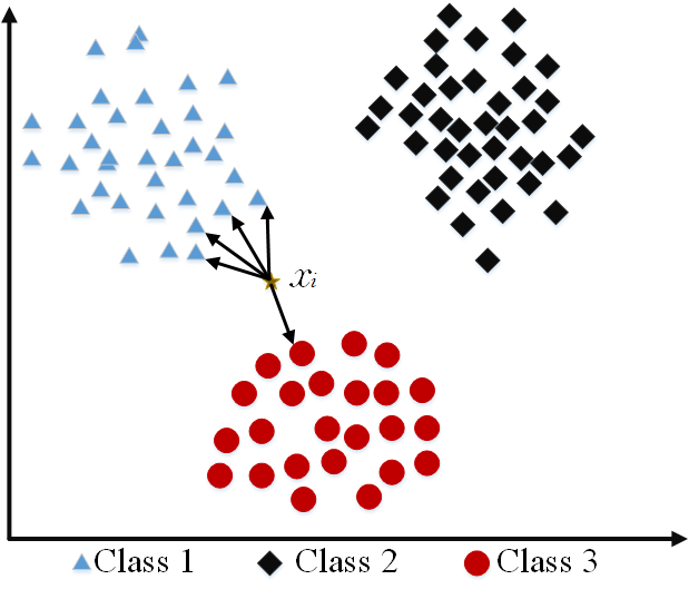
avg / total 0.82 0.77 0.77 7532R In machine learning, the k-nearest neighbors algorithm (kNN) is a non-parametric technique used for classification. This method is used in Natural-language processing (NLP) as a text classification technique in many researches in the past decades.
from sklearn.neighbors import KNeighborsClassifier
from sklearn.pipeline import Pipeline
from sklearn import metrics
from sklearn.feature_extraction.text import CountVectorizer
from sklearn.feature_extraction.text import TfidfTransformer
from sklearn.datasets import fetch_20newsgroups

newsgroups_train = fetch_20newsgroups(subset='train')
newsgroups_test = fetch_20newsgroups(subset='test')
X_train = newsgroups_train.data
X_test = newsgroups_test.data
y_train = newsgroups_train.target
y_test = newsgroups_test.target

text_clf = Pipeline([('vect', CountVectorizer()),
                     ('tfidf', TfidfTransformer()),
                     ('clf', KNeighborsClassifier()),
                     ])

text_clf.fit(X_train, y_train)

predicted = text_clf.predict(X_test)

print(metrics.classification_report(y_test, predicted))
Output:
               precision    recall  f1-score   support

          0       0.43      0.76      0.55       319
          1       0.50      0.61      0.55       389
          2       0.56      0.57      0.57       394
          3       0.53      0.58      0.56       392
          4       0.59      0.56      0.57       385
          5       0.69      0.60      0.64       395
          6       0.58      0.45      0.51       390
          7       0.75      0.69      0.72       396
          8       0.84      0.81      0.82       398
          9       0.77      0.72      0.74       397
         10       0.85      0.84      0.84       399
         11       0.76      0.84      0.80       396
         12       0.70      0.50      0.58       393
         13       0.82      0.49      0.62       396
         14       0.79      0.76      0.78       394
         15       0.75      0.76      0.76       398
         16       0.70      0.73      0.72       364
         17       0.62      0.76      0.69       376
         18       0.55      0.61      0.58       310
         19       0.56      0.49      0.52       251

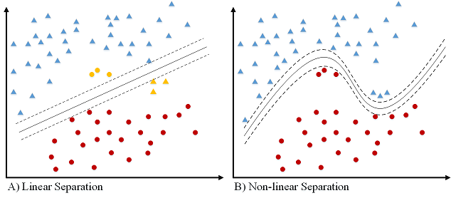
avg / total 0.67 0.66 0.66 7532The original version of SVM was introduced by Vapnik and Chervonenkis in 1963. The early 1990s, nonlinear version was addressed by BE. Boser et al.. Original version of SVM was designed for binary classification problem, but Many researchers have worked on multi-class problem using this authoritative technique.
The advantages of support vector machines are based on scikit-learn page:
- Effective in high dimensional spaces.
- Still effective in cases where number of dimensions is greater than the number of samples.
- Uses a subset of training points in the decision function (called support vectors), so it is also memory efficient.
- Versatile: different Kernel functions can be specified for the decision function. Common kernels are provided, but it is also possible to specify custom kernels.
The disadvantages of support vector machines include:
- If the number of features is much greater than the number of samples, avoiding over-fitting via choosing kernel functions and regularization term is crucial.
- SVMs do not directly provide probability estimates, these are calculated using an expensive five-fold cross-validation (see Scores and probabilities, below).
from sklearn.svm import LinearSVC
from sklearn.pipeline import Pipeline
from sklearn import metrics
from sklearn.feature_extraction.text import CountVectorizer
from sklearn.feature_extraction.text import TfidfTransformer
from sklearn.datasets import fetch_20newsgroups

newsgroups_train = fetch_20newsgroups(subset='train')
newsgroups_test = fetch_20newsgroups(subset='test')
X_train = newsgroups_train.data
X_test = newsgroups_test.data
y_train = newsgroups_train.target
y_test = newsgroups_test.target

text_clf = Pipeline([('vect', CountVectorizer()),
                     ('tfidf', TfidfTransformer()),
                     ('clf', LinearSVC()),
                     ])

text_clf.fit(X_train, y_train)


predicted = text_clf.predict(X_test)

print(metrics.classification_report(y_test, predicted))
output:
               precision    recall  f1-score   support

          0       0.82      0.80      0.81       319
          1       0.76      0.80      0.78       389
          2       0.77      0.73      0.75       394
          3       0.71      0.76      0.74       392
          4       0.84      0.86      0.85       385
          5       0.87      0.76      0.81       395
          6       0.83      0.91      0.87       390
          7       0.92      0.91      0.91       396
          8       0.95      0.95      0.95       398
          9       0.92      0.95      0.93       397
         10       0.96      0.98      0.97       399
         11       0.93      0.94      0.93       396
         12       0.81      0.79      0.80       393
         13       0.90      0.87      0.88       396
         14       0.90      0.93      0.92       394
         15       0.84      0.93      0.88       398
         16       0.75      0.92      0.82       364
         17       0.97      0.89      0.93       376
         18       0.82      0.62      0.71       310
         19       0.75      0.61      0.68       251

avg / total 0.85 0.85 0.85 7532One of earlier classification algorithm for text and data mining is decision tree. Decision tree classifiers (DTC's) are used successfully in many diverse areas of classification. The structure of this technique includes a hierarchical decomposition of the data space (only train dataset). Decision tree as classification task was introduced by D. Morgan and developed by JR. Quinlan. The main idea is creating trees based on the attributes of the data points, but the challenge is determining which attribute should be in parent level and which one should be in child level. To solve this problem, De Mantaras introduced statistical modeling for feature selection in tree.
from sklearn import tree
from sklearn.pipeline import Pipeline
from sklearn import metrics
from sklearn.feature_extraction.text import CountVectorizer
from sklearn.feature_extraction.text import TfidfTransformer
from sklearn.datasets import fetch_20newsgroups

newsgroups_train = fetch_20newsgroups(subset='train')
newsgroups_test = fetch_20newsgroups(subset='test')
X_train = newsgroups_train.data
X_test = newsgroups_test.data
y_train = newsgroups_train.target
y_test = newsgroups_test.target

text_clf = Pipeline([('vect', CountVectorizer()),
                     ('tfidf', TfidfTransformer()),
                     ('clf', tree.DecisionTreeClassifier()),
                     ])

text_clf.fit(X_train, y_train)


predicted = text_clf.predict(X_test)

print(metrics.classification_report(y_test, predicted))
output:
               precision    recall  f1-score   support

          0       0.51      0.48      0.49       319
          1       0.42      0.42      0.42       389
          2       0.51      0.56      0.53       394
          3       0.46      0.42      0.44       392
          4       0.50      0.56      0.53       385
          5       0.50      0.47      0.48       395
          6       0.66      0.73      0.69       390
          7       0.60      0.59      0.59       396
          8       0.66      0.72      0.69       398
          9       0.53      0.55      0.54       397
         10       0.68      0.66      0.67       399
         11       0.73      0.69      0.71       396
         12       0.34      0.33      0.33       393
         13       0.52      0.42      0.46       396
         14       0.65      0.62      0.63       394
         15       0.68      0.72      0.70       398
         16       0.49      0.62      0.55       364
         17       0.78      0.60      0.68       376
         18       0.38      0.38      0.38       310
         19       0.32      0.32      0.32       251

avg / total       0.55      0.55      0.55      7532
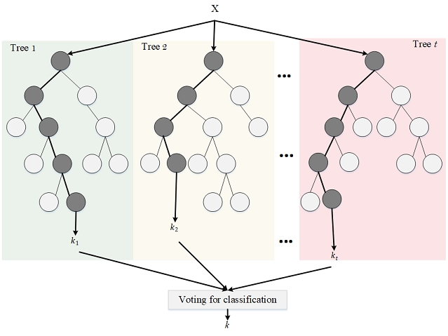
Random forests or random decision forests technique is an ensemble learning method for text classification. This method was introduced by T. Kam Ho in 1995 for first time which used t trees in parallel. This technique was later developed by L. Breiman in 1999 that they found converged for RF as a margin measure.
from sklearn.ensemble import RandomForestClassifier
from sklearn.pipeline import Pipeline
from sklearn import metrics
from sklearn.feature_extraction.text import CountVectorizer
from sklearn.feature_extraction.text import TfidfTransformer
from sklearn.datasets import fetch_20newsgroups

newsgroups_train = fetch_20newsgroups(subset='train')
newsgroups_test = fetch_20newsgroups(subset='test')
X_train = newsgroups_train.data
X_test = newsgroups_test.data
y_train = newsgroups_train.target
y_test = newsgroups_test.target

text_clf = Pipeline([('vect', CountVectorizer()),
                     ('tfidf', TfidfTransformer()),
                     ('clf', RandomForestClassifier(n_estimators=100)),
                     ])

text_clf.fit(X_train, y_train)


predicted = text_clf.predict(X_test)

print(metrics.classification_report(y_test, predicted))
output:
                precision    recall  f1-score   support

          0       0.69      0.63      0.66       319
          1       0.56      0.69      0.62       389
          2       0.67      0.78      0.72       394
          3       0.67      0.67      0.67       392
          4       0.71      0.78      0.74       385
          5       0.78      0.68      0.73       395
          6       0.74      0.92      0.82       390
          7       0.81      0.79      0.80       396
          8       0.90      0.89      0.90       398
          9       0.80      0.89      0.84       397
         10       0.90      0.93      0.91       399
         11       0.89      0.91      0.90       396
         12       0.68      0.49      0.57       393
         13       0.83      0.65      0.73       396
         14       0.81      0.88      0.84       394
         15       0.68      0.91      0.78       398
         16       0.67      0.86      0.75       364
         17       0.93      0.78      0.85       376
         18       0.86      0.48      0.61       310
         19       0.79      0.31      0.45       251

avg / total       0.77      0.76      0.75      7532
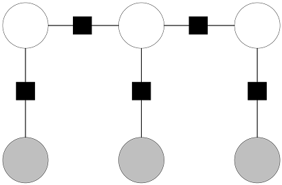
Conditional Random Field (CRF) is an undirected graphical model as shown in figure. CRFs state the conditional probability of a label sequence Y give a sequence of observation X i.e. P(Y|X). CRFs can incorporate complex features of observation sequence without violating the independence assumption by modeling the conditional probability of the label sequences rather than the joint probability P(X,Y). The concept of clique which is a fully connected subgraph and clique potential are used for computing P(X|Y). Considering one potential function for each clique of the graph, the probability of a variable configuration corresponds to the product of a series of non-negative potential function. The value computed by each potential function is equivalent to the probability of the variables in its corresponding clique taken on a particular configuration.
Example from Here Let’s use CoNLL 2002 data to build a NER system CoNLL2002 corpus is available in NLTK. We use Spanish data.
import nltk
import sklearn_crfsuite
from sklearn_crfsuite import metrics
nltk.corpus.conll2002.fileids()
train_sents = list(nltk.corpus.conll2002.iob_sents('esp.train'))
test_sents = list(nltk.corpus.conll2002.iob_sents('esp.testb'))
sklearn-crfsuite (and python-crfsuite) supports several feature formats; here we use feature dicts.
def word2features(sent, i):
    word = sent[i][0]
    postag = sent[i][1]

    features = {
        'bias': 1.0,
        'word.lower()': word.lower(),
        'word[-3:]': word[-3:],
        'word[-2:]': word[-2:],
        'word.isupper()': word.isupper(),
        'word.istitle()': word.istitle(),
        'word.isdigit()': word.isdigit(),
        'postag': postag,
        'postag[:2]': postag[:2],
    }
    if i > 0:
        word1 = sent[i-1][0]
        postag1 = sent[i-1][1]
        features.update({
            '-1:word.lower()': word1.lower(),
            '-1:word.istitle()': word1.istitle(),
            '-1:word.isupper()': word1.isupper(),
            '-1:postag': postag1,
            '-1:postag[:2]': postag1[:2],
        })
    else:
        features['BOS'] = True

    if i < len(sent)-1:
        word1 = sent[i+1][0]
        postag1 = sent[i+1][1]
        features.update({
            '+1:word.lower()': word1.lower(),
            '+1:word.istitle()': word1.istitle(),
            '+1:word.isupper()': word1.isupper(),
            '+1:postag': postag1,
            '+1:postag[:2]': postag1[:2],
        })
    else:
        features['EOS'] = True

    return features


def sent2features(sent):
    return [word2features(sent, i) for i in range(len(sent))]

def sent2labels(sent):
    return [label for token, postag, label in sent]

def sent2tokens(sent):
    return [token for token, postag, label in sent]

X_train = [sent2features(s) for s in train_sents]
y_train = [sent2labels(s) for s in train_sents]

X_test = [sent2features(s) for s in test_sents]
y_test = [sent2labels(s) for s in test_sents]
To see all possible CRF parameters check its docstring. Here we are useing L-BFGS training algorithm (it is default) with Elastic Net (L1 + L2) regularization.
crf = sklearn_crfsuite.CRF(
    algorithm='lbfgs',
    c1=0.1,
    c2=0.1,
    max_iterations=100,
    all_possible_transitions=True
)
crf.fit(X_train, y_train)
Evaluation
y_pred = crf.predict(X_test)
print(metrics.flat_classification_report(
    y_test, y_pred,  digits=3
))
Output:
               precision    recall  f1-score   support

      B-LOC      0.810     0.784     0.797      1084
     B-MISC      0.731     0.569     0.640       339
      B-ORG      0.807     0.832     0.820      1400
      B-PER      0.850     0.884     0.867       735
      I-LOC      0.690     0.637     0.662       325
     I-MISC      0.699     0.589     0.639       557
      I-ORG      0.852     0.786     0.818      1104
      I-PER      0.893     0.943     0.917       634
          O      0.992     0.997     0.994     45355

avg / total      0.970     0.971     0.971     51533
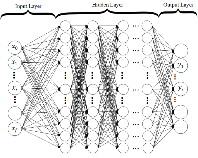
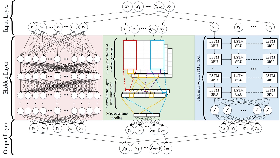
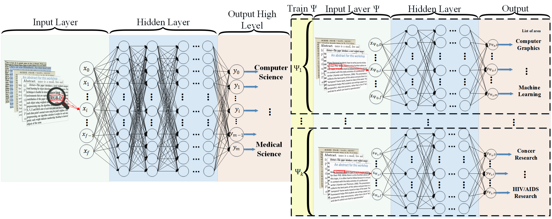
Deep Neural Networks architectures are designed to learn through multiple connection of layers where each single layer only receives connection from previous and provides connections only to the next layer in hidden part. The input is a connection of feature space (As discussed in Section Feature_extraction with first hidden layer. For Deep Neural Networks (DNN), input layer could be tf-ifd, word embedding, or etc. as shown in standard DNN in Figure. The output layer houses neurons equal to the number of classes for multi-class classification and only one neuron for binary classification. But our main contribution in this paper is that we have many trained DNNs to serve different purposes. Here, we have multi-class DNNs where each learning model is generated randomly (number of nodes in each layer as well as the number of layers are randomly assigned). Our implementation of Deep Neural Network (DNN) is basically a discriminatively trained model that uses standard back-propagation algorithm and sigmoid or ReLU as activation functions. The output layer for multi-class classification should use Softmax.
import packages:
from sklearn.datasets import fetch_20newsgroups
from keras.layers import  Dropout, Dense
from keras.models import Sequential
from sklearn.feature_extraction.text import TfidfVectorizer
import numpy as np
from sklearn import metrics
convert text to TF-IDF:
def TFIDF(X_train, X_test,MAX_NB_WORDS=75000):
    vectorizer_x = TfidfVectorizer(max_features=MAX_NB_WORDS)
    X_train = vectorizer_x.fit_transform(X_train).toarray()
    X_test = vectorizer_x.transform(X_test).toarray()
    print("tf-idf with",str(np.array(X_train).shape[1]),"features")
    return (X_train,X_test)
Build a DNN Model for Text:
def Build_Model_DNN_Text(shape, nClasses, dropout=0.5):
    """
    buildModel_DNN_Tex(shape, nClasses,dropout)
    Build Deep neural networks Model for text classification
    Shape is input feature space
    nClasses is number of classes
    """
    model = Sequential()
    node = 512 # number of nodes
    nLayers = 4 # number of  hidden layer

    model.add(Dense(node,input_dim=shape,activation='relu'))
    model.add(Dropout(dropout))
    for i in range(0,nLayers):
        model.add(Dense(node,input_dim=node,activation='relu'))
        model.add(Dropout(dropout))
    model.add(Dense(nClasses, activation='softmax'))

    model.compile(loss='sparse_categorical_crossentropy',
                  optimizer='adam',
                  metrics=['accuracy'])

    return model
Load text dataset (20newsgroups):
newsgroups_train = fetch_20newsgroups(subset='train')
newsgroups_test = fetch_20newsgroups(subset='test')
X_train = newsgroups_train.data
X_test = newsgroups_test.data
y_train = newsgroups_train.target
y_test = newsgroups_test.target
run DNN and see our result:
X_train_tfidf,X_test_tfidf = TFIDF(X_train,X_test)
model_DNN = Build_Model_DNN_Text(X_train_tfidf.shape[1], 20)
model_DNN.fit(X_train_tfidf, y_train,
                              validation_data=(X_test_tfidf, y_test),
                              epochs=10,
                              batch_size=128,
                              verbose=2)

predicted = model_DNN.predict_class(X_test_tfidf)

print(metrics.classification_report(y_test, predicted))
Model summary:
_________________________________________________________________
Layer (type)                 Output Shape              Param #
=================================================================
dense_1 (Dense)              (None, 512)               38400512
_________________________________________________________________
dropout_1 (Dropout)          (None, 512)               0
_________________________________________________________________
dense_2 (Dense)              (None, 512)               262656
_________________________________________________________________
dropout_2 (Dropout)          (None, 512)               0
_________________________________________________________________
dense_3 (Dense)              (None, 512)               262656
_________________________________________________________________
dropout_3 (Dropout)          (None, 512)               0
_________________________________________________________________
dense_4 (Dense)              (None, 512)               262656
_________________________________________________________________
dropout_4 (Dropout)          (None, 512)               0
_________________________________________________________________
dense_5 (Dense)              (None, 512)               262656
_________________________________________________________________
dropout_5 (Dropout)          (None, 512)               0
_________________________________________________________________
dense_6 (Dense)              (None, 20)                10260
=================================================================
Total params: 39,461,396
Trainable params: 39,461,396
Non-trainable params: 0
_________________________________________________________________
Output:
Train on 11314 samples, validate on 7532 samples
Epoch 1/10
 - 16s - loss: 2.7553 - acc: 0.1090 - val_loss: 1.9330 - val_acc: 0.3184
Epoch 2/10
 - 15s - loss: 1.5330 - acc: 0.4222 - val_loss: 1.1546 - val_acc: 0.6204
Epoch 3/10
 - 15s - loss: 0.7438 - acc: 0.7257 - val_loss: 0.8405 - val_acc: 0.7499
Epoch 4/10
 - 15s - loss: 0.2967 - acc: 0.9020 - val_loss: 0.9214 - val_acc: 0.7767
Epoch 5/10
 - 15s - loss: 0.1557 - acc: 0.9543 - val_loss: 0.8965 - val_acc: 0.7917
Epoch 6/10
 - 15s - loss: 0.1015 - acc: 0.9705 - val_loss: 0.9427 - val_acc: 0.7949
Epoch 7/10
 - 15s - loss: 0.0595 - acc: 0.9835 - val_loss: 0.9893 - val_acc: 0.7995
Epoch 8/10
 - 15s - loss: 0.0495 - acc: 0.9866 - val_loss: 0.9512 - val_acc: 0.8079
Epoch 9/10
 - 15s - loss: 0.0437 - acc: 0.9867 - val_loss: 0.9690 - val_acc: 0.8117
Epoch 10/10
 - 15s - loss: 0.0443 - acc: 0.9880 - val_loss: 1.0004 - val_acc: 0.8070


               precision    recall  f1-score   support

          0       0.76      0.78      0.77       319
          1       0.67      0.80      0.73       389
          2       0.82      0.63      0.71       394
          3       0.76      0.69      0.72       392
          4       0.65      0.86      0.74       385
          5       0.84      0.75      0.79       395
          6       0.82      0.87      0.84       390
          7       0.86      0.90      0.88       396
          8       0.95      0.91      0.93       398
          9       0.91      0.92      0.92       397
         10       0.98      0.92      0.95       399
         11       0.96      0.85      0.90       396
         12       0.71      0.69      0.70       393
         13       0.95      0.70      0.81       396
         14       0.86      0.91      0.88       394
         15       0.85      0.90      0.87       398
         16       0.79      0.84      0.81       364
         17       0.99      0.77      0.87       376
         18       0.58      0.75      0.65       310
         19       0.52      0.60      0.55       251

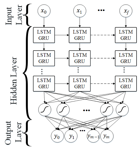
avg / total 0.82 0.81 0.81 7532Another neural network architecture that is addressed by the researchers for text miming and classification is Recurrent Neural Networks (RNN). RNN assigns more weights to the previous data points of sequence. Therefore, this technique is a powerful method for text, string and sequential data classification. Moreover, this technique could be used for image classification as we did in this work. In RNN, the neural net considers the information of previous nodes in a very sophisticated method which allows for better semantic analysis of the structures in the dataset.
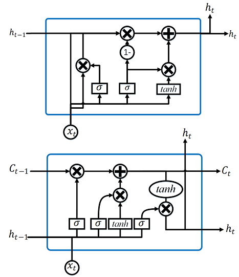
Gated Recurrent Unit (GRU) is a gating mechanism for RNN which was introduced by J. Chung et al. and K.Cho et al.. GRU is a simplified variant of the LSTM architecture, but there are differences as follows: GRU contains two gates and does not possess any internal memory (as shown in Figure; and finally, a second non-linearity is not applied (tanh in Figure).
Long Short-Term Memory~(LSTM) was introduced by S. Hochreiter and J. Schmidhuber and developed by many research scientists.
To deal with these problems Long Short-Term Memory (LSTM) is a special type of RNN that preserves long term dependency in a more effective way compared to the basic RNNs. This is particularly useful to overcome vanishing gradient problem. Although LSTM has a chain-like structure similar to RNN, LSTM uses multiple gates to carefully regulate the amount of information that will be allowed into each node state. Figure shows the basic cell of a LSTM model.
import packages:
from keras.layers import Dropout, Dense, GRU, Embedding
from keras.models import Sequential
from sklearn.feature_extraction.text import TfidfVectorizer
import numpy as np
from sklearn import metrics
from keras.preprocessing.text import Tokenizer
from keras.preprocessing.sequence import pad_sequences
from sklearn.datasets import fetch_20newsgroups
convert text to word embedding (Using GloVe):
def loadData_Tokenizer(X_train, X_test,MAX_NB_WORDS=75000,MAX_SEQUENCE_LENGTH=500):
    np.random.seed(7)
    text = np.concatenate((X_train, X_test), axis=0)
    text = np.array(text)
    tokenizer = Tokenizer(num_words=MAX_NB_WORDS)
    tokenizer.fit_on_texts(text)
    sequences = tokenizer.texts_to_sequences(text)
    word_index = tokenizer.word_index
    text = pad_sequences(sequences, maxlen=MAX_SEQUENCE_LENGTH)
    print('Found %s unique tokens.' % len(word_index))
    indices = np.arange(text.shape[0])
    # np.random.shuffle(indices)
    text = text[indices]
    print(text.shape)
    X_train = text[0:len(X_train), ]
    X_test = text[len(X_train):, ]
    embeddings_index = {}
    f = open(".\\Glove\\glove.6B.50d.txt", encoding="utf8")
    for line in f:

        values = line.split()
        word = values[0]
        try:
            coefs = np.asarray(values[1:], dtype='float32')
        except:
            pass
        embeddings_index[word] = coefs
    f.close()
    print('Total %s word vectors.' % len(embeddings_index))
    return (X_train, X_test, word_index,embeddings_index)
Build a RNN Model for Text:
def Build_Model_RNN_Text(word_index, embeddings_index, nclasses,  MAX_SEQUENCE_LENGTH=500, EMBEDDING_DIM=50, dropout=0.5):
    """
    def buildModel_RNN(word_index, embeddings_index, nclasses,  MAX_SEQUENCE_LENGTH=500, EMBEDDING_DIM=50, dropout=0.5):
    word_index in word index ,
    embeddings_index is embeddings index, look at data_helper.py
    nClasses is number of classes,
    MAX_SEQUENCE_LENGTH is maximum lenght of text sequences
    """

    model = Sequential()
    hidden_layer = 3
    gru_node = 32

    embedding_matrix = np.random.random((len(word_index) + 1, EMBEDDING_DIM))
    for word, i in word_index.items():
        embedding_vector = embeddings_index.get(word)
        if embedding_vector is not None:
            # words not found in embedding index will be all-zeros.
            if len(embedding_matrix[i]) != len(embedding_vector):
                print("could not broadcast input array from shape", str(len(embedding_matrix[i])),
                      "into shape", str(len(embedding_vector)), " Please make sure your"
                                                                " EMBEDDING_DIM is equal to embedding_vector file ,GloVe,")
                exit(1)
            embedding_matrix[i] = embedding_vector
    model.add(Embedding(len(word_index) + 1,
                                EMBEDDING_DIM,
                                weights=[embedding_matrix],
                                input_length=MAX_SEQUENCE_LENGTH,
                                trainable=True))


    print(gru_node)
    for i in range(0,hidden_layer):
        model.add(GRU(gru_node,return_sequences=True, recurrent_dropout=0.2))
        model.add(Dropout(dropout))
    model.add(GRU(gru_node, recurrent_dropout=0.2))
    model.add(Dropout(dropout))
    model.add(Dense(256, activation='relu'))
    model.add(Dense(nclasses, activation='softmax'))


    model.compile(loss='sparse_categorical_crossentropy',
                      optimizer='adam',
                      metrics=['accuracy'])
    return model
run RNN and see our result:
newsgroups_train = fetch_20newsgroups(subset='train')
newsgroups_test = fetch_20newsgroups(subset='test')
X_train = newsgroups_train.data
X_test = newsgroups_test.data
y_train = newsgroups_train.target
y_test = newsgroups_test.target

X_train_Glove,X_test_Glove, word_index,embeddings_index = loadData_Tokenizer(X_train,X_test)


model_RNN = Build_Model_RNN_Text(word_index,embeddings_index, 20)

model_RNN.fit(X_train_Glove, y_train,
                              validation_data=(X_test_Glove, y_test),
                              epochs=10,
                              batch_size=128,
                              verbose=2)

predicted = model_RNN.predict_classes(X_test_Glove)

print(metrics.classification_report(y_test, predicted))
Model summary:
_________________________________________________________________
Layer (type)                 Output Shape              Param #
=================================================================
embedding_1 (Embedding)      (None, 500, 50)           8960500
_________________________________________________________________
gru_1 (GRU)                  (None, 500, 256)          235776
_________________________________________________________________
dropout_1 (Dropout)          (None, 500, 256)          0
_________________________________________________________________
gru_2 (GRU)                  (None, 500, 256)          393984
_________________________________________________________________
dropout_2 (Dropout)          (None, 500, 256)          0
_________________________________________________________________
gru_3 (GRU)                  (None, 500, 256)          393984
_________________________________________________________________
dropout_3 (Dropout)          (None, 500, 256)          0
_________________________________________________________________
gru_4 (GRU)                  (None, 256)               393984
_________________________________________________________________
dense_1 (Dense)              (None, 20)                5140
=================================================================
Total params: 10,383,368
Trainable params: 10,383,368
Non-trainable params: 0
_________________________________________________________________
Output:
Train on 11314 samples, validate on 7532 samples
Epoch 1/20
 - 268s - loss: 2.5347 - acc: 0.1792 - val_loss: 2.2857 - val_acc: 0.2460
Epoch 2/20
 - 271s - loss: 1.6751 - acc: 0.3999 - val_loss: 1.4972 - val_acc: 0.4660
Epoch 3/20
 - 270s - loss: 1.0945 - acc: 0.6072 - val_loss: 1.3232 - val_acc: 0.5483
Epoch 4/20
 - 269s - loss: 0.7761 - acc: 0.7312 - val_loss: 1.1009 - val_acc: 0.6452
Epoch 5/20
 - 269s - loss: 0.5513 - acc: 0.8112 - val_loss: 1.0395 - val_acc: 0.6832
Epoch 6/20
 - 269s - loss: 0.3765 - acc: 0.8754 - val_loss: 0.9977 - val_acc: 0.7086
Epoch 7/20
 - 270s - loss: 0.2481 - acc: 0.9202 - val_loss: 1.0485 - val_acc: 0.7270
Epoch 8/20
 - 269s - loss: 0.1717 - acc: 0.9463 - val_loss: 1.0269 - val_acc: 0.7394
Epoch 9/20
 - 269s - loss: 0.1130 - acc: 0.9644 - val_loss: 1.1498 - val_acc: 0.7369
Epoch 10/20
 - 269s - loss: 0.0640 - acc: 0.9808 - val_loss: 1.1442 - val_acc: 0.7508
Epoch 11/20
 - 269s - loss: 0.0567 - acc: 0.9828 - val_loss: 1.2318 - val_acc: 0.7414
Epoch 12/20
 - 268s - loss: 0.0472 - acc: 0.9858 - val_loss: 1.2204 - val_acc: 0.7496
Epoch 13/20
 - 269s - loss: 0.0319 - acc: 0.9910 - val_loss: 1.1895 - val_acc: 0.7657
Epoch 14/20
 - 268s - loss: 0.0466 - acc: 0.9853 - val_loss: 1.2821 - val_acc: 0.7517
Epoch 15/20
 - 271s - loss: 0.0269 - acc: 0.9917 - val_loss: 1.2869 - val_acc: 0.7557
Epoch 16/20
 - 271s - loss: 0.0187 - acc: 0.9950 - val_loss: 1.3037 - val_acc: 0.7598
Epoch 17/20
 - 268s - loss: 0.0157 - acc: 0.9959 - val_loss: 1.2974 - val_acc: 0.7638
Epoch 18/20
 - 270s - loss: 0.0121 - acc: 0.9966 - val_loss: 1.3526 - val_acc: 0.7602
Epoch 19/20
 - 269s - loss: 0.0262 - acc: 0.9926 - val_loss: 1.4182 - val_acc: 0.7517
Epoch 20/20
 - 269s - loss: 0.0249 - acc: 0.9918 - val_loss: 1.3453 - val_acc: 0.7638


               precision    recall  f1-score   support

          0       0.71      0.71      0.71       319
          1       0.72      0.68      0.70       389
          2       0.76      0.62      0.69       394
          3       0.67      0.58      0.62       392
          4       0.68      0.67      0.68       385
          5       0.75      0.73      0.74       395
          6       0.82      0.74      0.78       390
          7       0.83      0.83      0.83       396
          8       0.81      0.90      0.86       398
          9       0.92      0.90      0.91       397
         10       0.91      0.94      0.93       399
         11       0.87      0.76      0.81       396
         12       0.57      0.70      0.63       393
         13       0.81      0.85      0.83       396
         14       0.74      0.93      0.82       394
         15       0.82      0.83      0.83       398
         16       0.74      0.78      0.76       364
         17       0.96      0.83      0.89       376
         18       0.64      0.60      0.62       310
         19       0.48      0.56      0.52       251

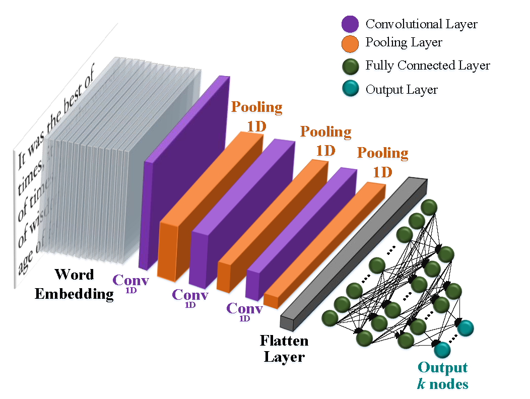
avg / total 0.77 0.76 0.76 7532Another deep learning architecture that is employed for hierarchical document classification is Convolutional Neural Networks (CNN) . Although originally built for image processing with architecture similar to the visual cortex, CNNs have also been effectively used for text classification. In a basic CNN for image processing, an image tensor is convolved with a set of kernels of size d by d. These convolution layers are called feature maps and can be stacked to provide multiple filters on the input. To reduce the computational complexity, CNNs use pooling which reduces the size of the output from one layer to the next in the network. Different pooling techniques are used to reduce outputs while preserving important features.
The most common pooling method is max pooling where the maximum element is selected from the pooling window. In order to feed the pooled output from stacked featured maps to the next layer, the maps are flattened into one column. The final layers in a CNN are typically fully connected dense layers. In general, during the back-propagation step of a convolutional neural network not only the weights are adjusted but also the feature detector filters. A potential problem of CNN used for text is the number of 'channels', Sigma (size of the feature space). This might be very large (e.g. 50K), for text but for images this is less of a problem (e.g. only 3 channels of RGB). This means the dimensionality of the CNN for text is very high.
import packages:
from keras.layers import Dropout, Dense,Input,Embedding,Flatten, MaxPooling1D, Conv1D
from keras.models import Sequential,Model
from sklearn.feature_extraction.text import TfidfVectorizer
import numpy as np
from sklearn import metrics
from keras.preprocessing.text import Tokenizer
from keras.preprocessing.sequence import pad_sequences
from sklearn.datasets import fetch_20newsgroups
from keras.layers.merge import Concatenate
convert text to word embedding (Using GloVe):
def loadData_Tokenizer(X_train, X_test,MAX_NB_WORDS=75000,MAX_SEQUENCE_LENGTH=500):
    np.random.seed(7)
    text = np.concatenate((X_train, X_test), axis=0)
    text = np.array(text)
    tokenizer = Tokenizer(num_words=MAX_NB_WORDS)
    tokenizer.fit_on_texts(text)
    sequences = tokenizer.texts_to_sequences(text)
    word_index = tokenizer.word_index
    text = pad_sequences(sequences, maxlen=MAX_SEQUENCE_LENGTH)
    print('Found %s unique tokens.' % len(word_index))
    indices = np.arange(text.shape[0])
    # np.random.shuffle(indices)
    text = text[indices]
    print(text.shape)
    X_train = text[0:len(X_train), ]
    X_test = text[len(X_train):, ]
    embeddings_index = {}
    f = open(".\\Glove\\glove.6B.50d.txt", encoding="utf8")
    for line in f:
        values = line.split()
        word = values[0]
        try:
            coefs = np.asarray(values[1:], dtype='float32')
        except:
            pass
        embeddings_index[word] = coefs
    f.close()
    print('Total %s word vectors.' % len(embeddings_index))
    return (X_train, X_test, word_index,embeddings_index)
Build a CNN Model for Text:
def Build_Model_CNN_Text(word_index, embeddings_index, nclasses, MAX_SEQUENCE_LENGTH=500, EMBEDDING_DIM=50, dropout=0.5):

    """
        def buildModel_CNN(word_index, embeddings_index, nclasses, MAX_SEQUENCE_LENGTH=500, EMBEDDING_DIM=50, dropout=0.5):
        word_index in word index ,
        embeddings_index is embeddings index, look at data_helper.py
        nClasses is number of classes,
        MAX_SEQUENCE_LENGTH is maximum lenght of text sequences,
        EMBEDDING_DIM is an int value for dimention of word embedding look at data_helper.py
    """

    model = Sequential()
    embedding_matrix = np.random.random((len(word_index) + 1, EMBEDDING_DIM))
    for word, i in word_index.items():
        embedding_vector = embeddings_index.get(word)
        if embedding_vector is not None:
            # words not found in embedding index will be all-zeros.
            if len(embedding_matrix[i]) !=len(embedding_vector):
                print("could not broadcast input array from shape",str(len(embedding_matrix[i])),
                                 "into shape",str(len(embedding_vector))," Please make sure your"
                                 " EMBEDDING_DIM is equal to embedding_vector file ,GloVe,")
                exit(1)

            embedding_matrix[i] = embedding_vector

    embedding_layer = Embedding(len(word_index) + 1,
                                EMBEDDING_DIM,
                                weights=[embedding_matrix],
                                input_length=MAX_SEQUENCE_LENGTH,
                                trainable=True)

    # applying a more complex convolutional approach
    convs = []
    filter_sizes = []
    layer = 5
    print("Filter  ",layer)
    for fl in range(0,layer):
        filter_sizes.append((fl+2))

    node = 128
    sequence_input = Input(shape=(MAX_SEQUENCE_LENGTH,), dtype='int32')
    embedded_sequences = embedding_layer(sequence_input)

    for fsz in filter_sizes:
        l_conv = Conv1D(node, kernel_size=fsz, activation='relu')(embedded_sequences)
        l_pool = MaxPooling1D(5)(l_conv)
        #l_pool = Dropout(0.25)(l_pool)
        convs.append(l_pool)

    l_merge = Concatenate(axis=1)(convs)
    l_cov1 = Conv1D(node, 5, activation='relu')(l_merge)
    l_cov1 = Dropout(dropout)(l_cov1)
    l_pool1 = MaxPooling1D(5)(l_cov1)
    l_cov2 = Conv1D(node, 5, activation='relu')(l_pool1)
    l_cov2 = Dropout(dropout)(l_cov2)
    l_pool2 = MaxPooling1D(30)(l_cov2)
    l_flat = Flatten()(l_pool2)
    l_dense = Dense(1024, activation='relu')(l_flat)
    l_dense = Dropout(dropout)(l_dense)
    l_dense = Dense(512, activation='relu')(l_dense)
    l_dense = Dropout(dropout)(l_dense)
    preds = Dense(nclasses, activation='softmax')(l_dense)
    model = Model(sequence_input, preds)

    model.compile(loss='sparse_categorical_crossentropy',
                  optimizer='adam',
                  metrics=['accuracy'])


    return model
run CNN and see our result:
newsgroups_train = fetch_20newsgroups(subset='train')
newsgroups_test = fetch_20newsgroups(subset='test')
X_train = newsgroups_train.data
X_test = newsgroups_test.data
y_train = newsgroups_train.target
y_test = newsgroups_test.target

X_train_Glove,X_test_Glove, word_index,embeddings_index = loadData_Tokenizer(X_train,X_test)


model_CNN = Build_Model_CNN_Text(word_index,embeddings_index, 20)


model_CNN.summary()

model_CNN.fit(X_train_Glove, y_train,
                              validation_data=(X_test_Glove, y_test),
                              epochs=15,
                              batch_size=128,
                              verbose=2)

predicted = model_CNN.predict(X_test_Glove)

predicted = np.argmax(predicted, axis=1)


print(metrics.classification_report(y_test, predicted))
Model:
__________________________________________________________________________________________________
Layer (type)                    Output Shape         Param #     Connected to
==================================================================================================
input_1 (InputLayer)            (None, 500)          0
__________________________________________________________________________________________________
embedding_1 (Embedding)         (None, 500, 50)      8960500     input_1[0][0]
__________________________________________________________________________________________________
conv1d_1 (Conv1D)               (None, 499, 128)     12928       embedding_1[0][0]
__________________________________________________________________________________________________
conv1d_2 (Conv1D)               (None, 498, 128)     19328       embedding_1[0][0]
__________________________________________________________________________________________________
conv1d_3 (Conv1D)               (None, 497, 128)     25728       embedding_1[0][0]
__________________________________________________________________________________________________
conv1d_4 (Conv1D)               (None, 496, 128)     32128       embedding_1[0][0]
__________________________________________________________________________________________________
conv1d_5 (Conv1D)               (None, 495, 128)     38528       embedding_1[0][0]
__________________________________________________________________________________________________
max_pooling1d_1 (MaxPooling1D)  (None, 99, 128)      0           conv1d_1[0][0]
__________________________________________________________________________________________________
max_pooling1d_2 (MaxPooling1D)  (None, 99, 128)      0           conv1d_2[0][0]
__________________________________________________________________________________________________
max_pooling1d_3 (MaxPooling1D)  (None, 99, 128)      0           conv1d_3[0][0]
__________________________________________________________________________________________________
max_pooling1d_4 (MaxPooling1D)  (None, 99, 128)      0           conv1d_4[0][0]
__________________________________________________________________________________________________
max_pooling1d_5 (MaxPooling1D)  (None, 99, 128)      0           conv1d_5[0][0]
__________________________________________________________________________________________________
concatenate_1 (Concatenate)     (None, 495, 128)     0           max_pooling1d_1[0][0]
                                                                 max_pooling1d_2[0][0]
                                                                 max_pooling1d_3[0][0]
                                                                 max_pooling1d_4[0][0]
                                                                 max_pooling1d_5[0][0]
__________________________________________________________________________________________________
conv1d_6 (Conv1D)               (None, 491, 128)     82048       concatenate_1[0][0]
__________________________________________________________________________________________________
dropout_1 (Dropout)             (None, 491, 128)     0           conv1d_6[0][0]
__________________________________________________________________________________________________
max_pooling1d_6 (MaxPooling1D)  (None, 98, 128)      0           dropout_1[0][0]
__________________________________________________________________________________________________
conv1d_7 (Conv1D)               (None, 94, 128)      82048       max_pooling1d_6[0][0]
__________________________________________________________________________________________________
dropout_2 (Dropout)             (None, 94, 128)      0           conv1d_7[0][0]
__________________________________________________________________________________________________
max_pooling1d_7 (MaxPooling1D)  (None, 3, 128)       0           dropout_2[0][0]
__________________________________________________________________________________________________
flatten_1 (Flatten)             (None, 384)          0           max_pooling1d_7[0][0]
__________________________________________________________________________________________________
dense_1 (Dense)                 (None, 1024)         394240      flatten_1[0][0]
__________________________________________________________________________________________________
dropout_3 (Dropout)             (None, 1024)         0           dense_1[0][0]
__________________________________________________________________________________________________
dense_2 (Dense)                 (None, 512)          524800      dropout_3[0][0]
__________________________________________________________________________________________________
dropout_4 (Dropout)             (None, 512)          0           dense_2[0][0]
__________________________________________________________________________________________________
dense_3 (Dense)                 (None, 20)           10260       dropout_4[0][0]
==================================================================================================
Total params: 10,182,536
Trainable params: 10,182,536
Non-trainable params: 0
__________________________________________________________________________________________________
Output:
Train on 11314 samples, validate on 7532 samples
Epoch 1/15
 - 6s - loss: 2.9329 - acc: 0.0783 - val_loss: 2.7628 - val_acc: 0.1403
Epoch 2/15
 - 4s - loss: 2.2534 - acc: 0.2249 - val_loss: 2.1715 - val_acc: 0.4007
Epoch 3/15
 - 4s - loss: 1.5643 - acc: 0.4326 - val_loss: 1.7846 - val_acc: 0.5052
Epoch 4/15
 - 4s - loss: 1.1771 - acc: 0.5662 - val_loss: 1.4949 - val_acc: 0.6131
Epoch 5/15
 - 4s - loss: 0.8880 - acc: 0.6797 - val_loss: 1.3629 - val_acc: 0.6256
Epoch 6/15
 - 4s - loss: 0.6990 - acc: 0.7569 - val_loss: 1.2013 - val_acc: 0.6624
Epoch 7/15
 - 4s - loss: 0.5037 - acc: 0.8200 - val_loss: 1.0674 - val_acc: 0.6807
Epoch 8/15
 - 4s - loss: 0.4050 - acc: 0.8626 - val_loss: 1.0223 - val_acc: 0.6863
Epoch 9/15
 - 4s - loss: 0.2952 - acc: 0.8968 - val_loss: 0.9045 - val_acc: 0.7120
Epoch 10/15
 - 4s - loss: 0.2314 - acc: 0.9217 - val_loss: 0.8574 - val_acc: 0.7326
Epoch 11/15
 - 4s - loss: 0.1778 - acc: 0.9436 - val_loss: 0.8752 - val_acc: 0.7270
Epoch 12/15
 - 4s - loss: 0.1475 - acc: 0.9524 - val_loss: 0.8299 - val_acc: 0.7355
Epoch 13/15
 - 4s - loss: 0.1089 - acc: 0.9657 - val_loss: 0.8034 - val_acc: 0.7491
Epoch 14/15
 - 4s - loss: 0.1047 - acc: 0.9666 - val_loss: 0.8172 - val_acc: 0.7463
Epoch 15/15
 - 4s - loss: 0.0749 - acc: 0.9774 - val_loss: 0.8511 - val_acc: 0.7313


               precision    recall  f1-score   support

          0       0.75      0.61      0.67       319
          1       0.63      0.74      0.68       389
          2       0.74      0.54      0.62       394
          3       0.49      0.76      0.60       392
          4       0.60      0.70      0.64       385
          5       0.79      0.57      0.66       395
          6       0.73      0.76      0.74       390
          7       0.83      0.74      0.78       396
          8       0.86      0.88      0.87       398
          9       0.95      0.78      0.86       397
         10       0.93      0.93      0.93       399
         11       0.92      0.77      0.84       396
         12       0.55      0.72      0.62       393
         13       0.76      0.85      0.80       396
         14       0.86      0.83      0.84       394
         15       0.91      0.73      0.81       398
         16       0.75      0.65      0.70       364
         17       0.95      0.86      0.90       376
         18       0.60      0.49      0.54       310
         19       0.37      0.60      0.46       251

avg / total 0.76 0.73 0.74 7532Recurrent Convolutional Neural Networks (RCNN) is also used for text classification. The main idea of this technique is capturing contextual information with the recurrent structure and constructing the representation of text using a convolutional neural network. This architecture is a combination of RNN and CNN to use advantages of both technique in a model.
import packages:
from keras.preprocessing import sequence
from keras.models import Sequential
from keras.layers import Dense, Dropout, Activation
from keras.layers import Embedding
from keras.layers import GRU
from keras.layers import Conv1D, MaxPooling1D
from keras.datasets import imdb
from sklearn.datasets import fetch_20newsgroups
import numpy as np
from sklearn import metrics
from keras.preprocessing.text import Tokenizer
from keras.preprocessing.sequence import pad_sequences
Convert text to word embedding (Using GloVe):
def loadData_Tokenizer(X_train, X_test,MAX_NB_WORDS=75000,MAX_SEQUENCE_LENGTH=500):
    np.random.seed(7)
    text = np.concatenate((X_train, X_test), axis=0)
    text = np.array(text)
    tokenizer = Tokenizer(num_words=MAX_NB_WORDS)
    tokenizer.fit_on_texts(text)
    sequences = tokenizer.texts_to_sequences(text)
    word_index = tokenizer.word_index
    text = pad_sequences(sequences, maxlen=MAX_SEQUENCE_LENGTH)
    print('Found %s unique tokens.' % len(word_index))
    indices = np.arange(text.shape[0])
    # np.random.shuffle(indices)
    text = text[indices]
    print(text.shape)
    X_train = text[0:len(X_train), ]
    X_test = text[len(X_train):, ]
    embeddings_index = {}
    f = open("C:\\Users\\kamran\\Documents\\GitHub\\RMDL\\Examples\\Glove\\glove.6B.50d.txt", encoding="utf8")
    for line in f:
        values = line.split()
        word = values[0]
        try:
            coefs = np.asarray(values[1:], dtype='float32')
        except:
            pass
        embeddings_index[word] = coefs
    f.close()
    print('Total %s word vectors.' % len(embeddings_index))
    return (X_train, X_test, word_index,embeddings_index)
def Build_Model_RCNN_Text(word_index, embeddings_index, nclasses, MAX_SEQUENCE_LENGTH=500, EMBEDDING_DIM=50):
kernel_size = 2
filters = 256
pool_size = 2
gru_node = 256
embedding_matrix = np.random.random((len(word_index) + 1, EMBEDDING_DIM))
for word, i in word_index.items():
embedding_vector = embeddings_index.get(word)
if embedding_vector is not None:
# words not found in embedding index will be all-zeros.
if len(embedding_matrix[i]) !=len(embedding_vector):
print("could not broadcast input array from shape",str(len(embedding_matrix[i])),
"into shape",str(len(embedding_vector))," Please make sure your"
" EMBEDDING_DIM is equal to embedding_vector file ,GloVe,")
exit(1)
embedding_matrix[i] = embedding_vector
model = Sequential()
model.add(Embedding(len(word_index) + 1,
EMBEDDING_DIM,
weights=[embedding_matrix],
input_length=MAX_SEQUENCE_LENGTH,
trainable=True))
model.add(Dropout(0.25))
model.add(Conv1D(filters, kernel_size, activation='relu'))
model.add(MaxPooling1D(pool_size=pool_size))
model.add(Conv1D(filters, kernel_size, activation='relu'))
model.add(MaxPooling1D(pool_size=pool_size))
model.add(Conv1D(filters, kernel_size, activation='relu'))
model.add(MaxPooling1D(pool_size=pool_size))
model.add(Conv1D(filters, kernel_size, activation='relu'))
model.add(MaxPooling1D(pool_size=pool_size))
model.add(LSTM(gru_node, return_sequences=True, recurrent_dropout=0.2))
model.add(LSTM(gru_node, return_sequences=True, recurrent_dropout=0.2))
model.add(LSTM(gru_node, return_sequences=True, recurrent_dropout=0.2))
model.add(LSTM(gru_node, recurrent_dropout=0.2))
model.add(Dense(1024,activation='relu'))
model.add(Dense(nclasses))
model.add(Activation('softmax'))
model.compile(loss='sparse_categorical_crossentropy',
optimizer='adam',
metrics=['accuracy'])
return modelnewsgroups_train = fetch_20newsgroups(subset='train')
newsgroups_test = fetch_20newsgroups(subset='test')
X_train = newsgroups_train.data
X_test = newsgroups_test.data
y_train = newsgroups_train.target
y_test = newsgroups_test.target
X_train_Glove,X_test_Glove, word_index,embeddings_index = loadData_Tokenizer(X_train,X_test)Run RCNN :
model_RCNN = Build_Model_CNN_Text(word_index,embeddings_index, 20)


model_RCNN.summary()

model_RCNN.fit(X_train_Glove, y_train,
                              validation_data=(X_test_Glove, y_test),
                              epochs=15,
                              batch_size=128,
                              verbose=2)

predicted = model_RCNN.predict(X_test_Glove)

predicted = np.argmax(predicted, axis=1)
print(metrics.classification_report(y_test, predicted))
summary of the model:
_________________________________________________________________
Layer (type)                 Output Shape              Param #
=================================================================
embedding_1 (Embedding)      (None, 500, 50)           8960500
_________________________________________________________________
dropout_1 (Dropout)          (None, 500, 50)           0
_________________________________________________________________
conv1d_1 (Conv1D)            (None, 499, 256)          25856
_________________________________________________________________
max_pooling1d_1 (MaxPooling1 (None, 249, 256)          0
_________________________________________________________________
conv1d_2 (Conv1D)            (None, 248, 256)          131328
_________________________________________________________________
max_pooling1d_2 (MaxPooling1 (None, 124, 256)          0
_________________________________________________________________
conv1d_3 (Conv1D)            (None, 123, 256)          131328
_________________________________________________________________
max_pooling1d_3 (MaxPooling1 (None, 61, 256)           0
_________________________________________________________________
conv1d_4 (Conv1D)            (None, 60, 256)           131328
_________________________________________________________________
max_pooling1d_4 (MaxPooling1 (None, 30, 256)           0
_________________________________________________________________
lstm_1 (LSTM)                (None, 30, 256)           525312
_________________________________________________________________
lstm_2 (LSTM)                (None, 30, 256)           525312
_________________________________________________________________
lstm_3 (LSTM)                (None, 30, 256)           525312
_________________________________________________________________
lstm_4 (LSTM)                (None, 256)               525312
_________________________________________________________________
dense_1 (Dense)              (None, 1024)              263168
_________________________________________________________________
dense_2 (Dense)              (None, 20)                20500
_________________________________________________________________
activation_1 (Activation)    (None, 20)                0
=================================================================
Total params: 11,765,256
Trainable params: 11,765,256
Non-trainable params: 0
_________________________________________________________________
Output:
Train on 11314 samples, validate on 7532 samples
Epoch 1/15
 - 28s - loss: 2.6624 - acc: 0.1081 - val_loss: 2.3012 - val_acc: 0.1753
Epoch 2/15
 - 22s - loss: 2.1142 - acc: 0.2224 - val_loss: 1.9168 - val_acc: 0.2669
Epoch 3/15
 - 22s - loss: 1.7465 - acc: 0.3290 - val_loss: 1.8257 - val_acc: 0.3412
Epoch 4/15
 - 22s - loss: 1.4730 - acc: 0.4356 - val_loss: 1.5433 - val_acc: 0.4436
Epoch 5/15
 - 22s - loss: 1.1800 - acc: 0.5556 - val_loss: 1.2973 - val_acc: 0.5467
Epoch 6/15
 - 22s - loss: 0.9910 - acc: 0.6281 - val_loss: 1.2530 - val_acc: 0.5797
Epoch 7/15
 - 22s - loss: 0.8581 - acc: 0.6854 - val_loss: 1.1522 - val_acc: 0.6281
Epoch 8/15
 - 22s - loss: 0.7058 - acc: 0.7428 - val_loss: 1.2385 - val_acc: 0.6033
Epoch 9/15
 - 22s - loss: 0.6792 - acc: 0.7515 - val_loss: 1.0200 - val_acc: 0.6775
Epoch 10/15
 - 22s - loss: 0.5782 - acc: 0.7948 - val_loss: 1.0961 - val_acc: 0.6577
Epoch 11/15
 - 23s - loss: 0.4674 - acc: 0.8341 - val_loss: 1.0866 - val_acc: 0.6924
Epoch 12/15
 - 23s - loss: 0.4284 - acc: 0.8512 - val_loss: 0.9880 - val_acc: 0.7096
Epoch 13/15
 - 22s - loss: 0.3883 - acc: 0.8670 - val_loss: 1.0190 - val_acc: 0.7151
Epoch 14/15
 - 22s - loss: 0.3334 - acc: 0.8874 - val_loss: 1.0025 - val_acc: 0.7232
Epoch 15/15
 - 22s - loss: 0.2857 - acc: 0.9038 - val_loss: 1.0123 - val_acc: 0.7331


             precision    recall  f1-score   support

          0       0.64      0.73      0.68       319
          1       0.45      0.83      0.58       389
          2       0.81      0.64      0.71       394
          3       0.64      0.57      0.61       392
          4       0.55      0.78      0.64       385
          5       0.77      0.52      0.62       395
          6       0.84      0.77      0.80       390
          7       0.87      0.79      0.83       396
          8       0.85      0.90      0.87       398
          9       0.98      0.84      0.90       397
         10       0.93      0.96      0.95       399
         11       0.92      0.79      0.85       396
         12       0.59      0.53      0.56       393
         13       0.82      0.82      0.82       396
         14       0.84      0.84      0.84       394
         15       0.83      0.89      0.86       398
         16       0.68      0.86      0.76       364
         17       0.97      0.86      0.91       376
         18       0.66      0.50      0.57       310
         19       0.53      0.31      0.40       251

avg / total 0.77 0.75 0.75 7532Referenced paper : RMDL: Random Multimodel Deep Learning for Classification
A new ensemble, deep learning approach for classification. Deep learning models have achieved state-of-the-art results across many domains. RMDL solves the problem of finding the best deep learning structure and architecture while simultaneously improving robustness and accuracy through ensembles of different deep learning architectures. RDMLs can accept a variety of data as input including text, video, images, and symbols.
Random Multimodel Deep Learning (RDML) architecture for classification. RMDL includes 3 Random models, oneDNN classifier at left, one Deep CNN classifier at middle, and one Deep RNN classifier at right (each unit could be LSTMor GRU).
Installation
There are pip and git for RMDL installation:
Using pip
pip install RMDLUsing git
git clone --recursive https://github.com/kk7nc/RMDL.gitThe primary requirements for this package are Python 3 with Tensorflow. The requirements.txt file contains a listing of the required Python packages; to install all requirements, run the following:
pip -r install requirements.txtOr
pip3 install -r requirements.txtOr:
conda install --file requirements.txtDocumentation:
The exponential growth in the number of complex datasets every year requires more enhancement in machine learning methods to provide robust and accurate data classification. Lately, deep learning approaches are achieving better results compared to previous machine learning algorithms on tasks like image classification, natural language processing, face recognition, and etc. The success of these deep learning algorithms rely on their capacity to model complex and non-linear relationships within the data. However, finding suitable structures for these models has been a challenge for researchers. This paper introduces Random Multimodel Deep Learning (RMDL): a new ensemble, deep learning approach for classification. RMDL aims to solve the problem of finding the best deep learning architecture while simultaneously improving the robustness and accuracy through ensembles of multiple deep learning architectures. In short, RMDL trains multiple models of Deep Neural Network (DNN), Convolutional Neural Network (CNN) and Recurrent Neural Network (RNN) in parallel and combines their results to produce better result of any of those models individually. To create these models, each deep learning model has been constructed in a random fashion regarding the number of layers and nodes in their neural network structure. The resulting RDML model can be used in various domains such as text, video, images, and symbolic. In this Project, we describe RMDL model in depth and show the results for image and text classification as well as face recognition. For image classification, we compared our model with some of the available baselines using MNIST and CIFAR-10 datasets. Similarly, we used four datasets namely, WOS, Reuters, IMDB, and 20newsgroup and compared our results with available baselines. Web of Science (WOS) has been collected by authors and consists of three sets~(small, medium and large set). Lastly, we used ORL dataset to compare the performance of our approach with other face recognition methods. These test results show that RDML model consistently outperform standard methods over a broad range of data types and classification problems.
Refrenced paper : HDLTex: Hierarchical Deep Learning for Text Classification
Documentation:
Increasingly large document collections require improved information processing methods for searching, retrieving, and organizing text documents. Central to these information processing methods is document classification, which has become an important task supervised learning aims to solve. Recently, the performance of traditional supervised classifiers has degraded as the number of documents has increased. This exponential growth of document volume has also increated the number of categories. This paper approaches this problem differently from current document classification methods that view the problem as multi-class classification. Instead we perform hierarchical classification using an approach we call Hierarchical Deep Learning for Text classification (HDLTex). HDLTex employs stacks of deep learning architectures to provide hierarchical understanding of the documents.
| Model | Advantages | Disadvantages |
| Rocchio Algorithm |
|
|
| Boosting and Bagging |
|
|
| Logistic Regression |
|
|
| Naive Bayes Classifier |
|
|
| K-Nearest Neighbor |
|
|
| Support Vector Machine (SVM) |
|
|
| Decision Tree |
|
|
| Conditional Random Field (CRF) |
|
|
| Random Forest |
|
|
| Deep Learning |
|
|
Compute the Matthews correlation coefficient (MCC)
The Matthews correlation coefficient is used in machine learning as a measure of the quality of binary (two-class) classification problems. It takes into account of true and false positives and negatives and is generally regarded as a balanced measure which can be used even if the classes are of very different sizes. The MCC is in essence a correlation coefficient value between -1 and +1. A coefficient of +1 represents a perfect prediction, 0 an average random prediction and -1 an inverse prediction. The statistic is also known as the phi coefficient.
from sklearn.metrics import matthews_corrcoef
y_true = [+1, +1, +1, -1]
y_pred = [+1, -1, +1, +1]
matthews_corrcoef(y_true, y_pred)ROC curves are typically used in binary classification to study the output of a classifier. In order to extend ROC curve and ROC area to multi-class or multi-label classification, it is necessary to binarize the output. One ROC curve can be drawn per label, but one can also draw a ROC curve by considering each element of the label indicator matrix as a binary prediction (micro-averaging).
Another evaluation measure for multi-class classification is macro-averaging, which gives equal weight to the classification of each label. [sources]
import numpy as np
import matplotlib.pyplot as plt
from itertools import cycle

from sklearn import svm, datasets
from sklearn.metrics import roc_curve, auc
from sklearn.model_selection import train_test_split
from sklearn.preprocessing import label_binarize
from sklearn.multiclass import OneVsRestClassifier
from scipy import interp

# Import some data to play with
iris = datasets.load_iris()
X = iris.data
y = iris.target

# Binarize the output
y = label_binarize(y, classes=[0, 1, 2])
n_classes = y.shape[1]

# Add noisy features to make the problem harder
random_state = np.random.RandomState(0)
n_samples, n_features = X.shape
X = np.c_[X, random_state.randn(n_samples, 200 * n_features)]

# shuffle and split training and test sets
X_train, X_test, y_train, y_test = train_test_split(X, y, test_size=.5,
                                                    random_state=0)

# Learn to predict each class against the other
classifier = OneVsRestClassifier(svm.SVC(kernel='linear', probability=True,
                                 random_state=random_state))
y_score = classifier.fit(X_train, y_train).decision_function(X_test)

# Compute ROC curve and ROC area for each class
fpr = dict()
tpr = dict()
roc_auc = dict()
for i in range(n_classes):
    fpr[i], tpr[i], _ = roc_curve(y_test[:, i], y_score[:, i])
    roc_auc[i] = auc(fpr[i], tpr[i])

# Compute micro-average ROC curve and ROC area
fpr["micro"], tpr["micro"], _ = roc_curve(y_test.ravel(), y_score.ravel())
roc_auc["micro"] = auc(fpr["micro"], tpr["micro"])
Plot of a ROC curve for a specific class
plt.figure()
lw = 2
plt.plot(fpr[2], tpr[2], color='darkorange',
         lw=lw, label='ROC curve (area = %0.2f)' % roc_auc[2])
plt.plot([0, 1], [0, 1], color='navy', lw=lw, linestyle='--')
plt.xlim([0.0, 1.0])
plt.ylim([0.0, 1.05])
plt.xlabel('False Positive Rate')
plt.ylabel('True Positive Rate')
plt.title('Receiver operating characteristic example')
plt.legend(loc="lower right")
plt.show()
Area under ROC curve (AUC) is a summary metric that measures the entire area underneath the ROC curve. AUC holds helpful properties, such as increased sensitivity in the analysis of variance (ANOVA) tests, independence of decision threshold, invariance to a priori class probability and the indication of how well negative and positive classes are regarding decision index.
import numpy as np
from sklearn import metrics
fpr, tpr, thresholds = metrics.roc_curve(y, pred, pos_label=2)
metrics.auc(fpr, tpr)Dataset of 25,000 movies reviews from IMDB, labeled by sentiment (positive/negative). Reviews have been preprocessed, and each review is encoded as a sequence of word indexes (integers). For convenience, words are indexed by overall frequency in the dataset, so that for instance the integer "3" encodes the 3rd most frequent word in the data. This allows for quick filtering operations, such as "only consider the top 10,000 most common words, but eliminate the top 20 most common words".
As a convention, "0" does not stand for a specific word, but instead is used to encode any unknown word.
from keras.datasets import imdb

(x_train, y_train), (x_test, y_test) = imdb.load_data(path="imdb.npz",
                                                      num_words=None,
                                                      skip_top=0,
                                                      maxlen=None,
                                                      seed=113,
                                                      start_char=1,
                                                      oov_char=2,
index_from=3)Dataset of 11,228 newswires from Reuters, labeled over 46 topics. As with the IMDB dataset, each wire is encoded as a sequence of word indexes (same conventions).
from keras.datasets import reuters

(x_train, y_train), (x_test, y_test) = reuters.load_data(path="reuters.npz",
                                                         num_words=None,
                                                         skip_top=0,
                                                         maxlen=None,
                                                         test_split=0.2,
                                                         seed=113,
                                                         start_char=1,
                                                         oov_char=2,
index_from=3)The 20 newsgroups dataset comprises around 18000 newsgroups posts on 20 topics split in two subsets: one for training (or development) and the other one for testing (or for performance evaluation). The split between the train and test set is based upon messages posted before and after a specific date.
This module contains two loaders. The first one, sklearn.datasets.fetch_20newsgroups, returns a list of the raw texts that can be fed to text feature extractors, such as sklearn.feature_extraction.text.CountVectorizer with custom parameters so as to extract feature vectors. The second one, sklearn.datasets.fetch_20newsgroups_vectorized, returns ready-to-use features, i.e., it is not necessary to use a feature extractor.
from sklearn.datasets import fetch_20newsgroups
newsgroups_train = fetch_20newsgroups(subset='train')

from pprint import pprint
pprint(list(newsgroups_train.target_names))

['alt.atheism',
 'comp.graphics',
 'comp.os.ms-windows.misc',
 'comp.sys.ibm.pc.hardware',
 'comp.sys.mac.hardware',
 'comp.windows.x',
 'misc.forsale',
 'rec.autos',
 'rec.motorcycles',
 'rec.sport.baseball',
 'rec.sport.hockey',
 'sci.crypt',
 'sci.electronics',
 'sci.med',
 'sci.space',
 'soc.religion.christian',
 'talk.politics.guns',
 'talk.politics.mideast',
 'talk.politics.misc',
'talk.religion.misc']Description of Dataset:
Here is three datasets which include WOS-11967 , WOS-46985, and WOS-5736 Each folder contains:
- X.txt
- Y.txt
- YL1.txt
- YL2.txt
X is input data that include text sequences Y is target value YL1 is target value of level one (parent label) YL2 is target value of level one (child label)
Meta-data: This folder contain on data file as following attribute: Y1 Y2 Y Domain area keywords Abstract
Abstract is input data that include text sequences of 46,985 published paper Y is target value YL1 is target value of level one (parent label) YL2 is target value of level one (child label) Domain is majaor domain which include 7 labales: {Computer Science,Electrical Engineering, Psychology, Mechanical Engineering,Civil Engineering, Medical Science, biochemistry} area is subdomain or area of the paper, such as CS-> computer graphics which contain 134 labels. keywords : is authors keyword of the papers
- Web of Science Dataset WOS-11967
This dataset contains 11,967 documents with 35 categories which include 7 parents categories.
- Web of Science Dataset WOS-46985
This dataset contains 46,985 documents with 134 categories which include 7 parents categories.
- Web of Science Dataset WOS-5736
This dataset contains 5,736 documents with 11 categories which include 3 parents categories.
Referenced paper: HDLTex: Hierarchical Deep Learning for Text Classification
Information retrieval is finding documents of an unstructured data that meet an information need from within large collections of documents. With the rapid growth of online information, particularly in text format, text classification has become a significant technique for managing this type of data. Some of the important methods used in this area are Naive Bayes, SVM, decision tree, J48, k-NN and IBK. One of the most challenging applications for document and text dataset processing is applying document categorization methods for information retrieval.
- 🎓 Introduction to information retrieval Manning, C., Raghavan, P., & Schütze, H. (2010).
- 🎓 Web forum retrieval and text analytics: A survey Hoogeveen, Doris, et al.. (2018).
- 🎓 Automatic Text Classification in Information retrieval: A Survey Dwivedi, Sanjay K., and Chandrakala Arya.. (2016).
Information filtering refers to selection of relevant information or rejection of irrelevant information from a stream of incoming data. Information filtering systems are typically used to measure and forecast users' long-term interests. Probabilistic models, such as Bayesian inference network, are commonly used in information filtering systems. Bayesian inference networks employ recursive inference to propagate values through the inference network and return documents with the highest ranking. Chris used vector space model with iterative refinement for filtering task.
- 🎓 Search engines: Information retrieval in practice Croft, W. B., Metzler, D., & Strohman, T. (2010).
- 🎓 Implementation of the SMART information retrieval system Buckley, Chris
Sentiment analysis is a computational approach toward identifying opinion, sentiment, and subjectivity in text. Sentiment classification methods classify a document associated with an opinion to be positive or negative. The assumption is that document d is expressing an opinion on a single entity e and opinions are formed via a single opinion holder h. Naive Bayesian classification and SVM are some of the most popular supervised learning methods that have been used for sentiment classification. Features such as terms and their respective frequency, part of speech, opinion words and phrases, negations and syntactic dependency have been used in sentiment classification techniques.
- 🎓 Opinion mining and sentiment analysis Pang, Bo, and Lillian Lee. (2008).
- 🎓 A survey of opinion mining and sentiment analysis Liu, Bing, and Lei Zhang. (2010).
- 🎓 Thumbs up?: sentiment classification using machine learning techniques Pang, Bo, Lillian Lee, and Shivakumar Vaithyanathan.
Content-based recommender systems suggest items to users based on the description of an item and a profile of the user's interests. A user's profile can be learned from user feedback (history of the search queries or self reports) on items as well as self-explained features~(filter or conditions on the queries) in one's profile. In this way, input to such recommender systems can be semi-structured such that some attributes are extracted from free-text field while others are directly specified. Many different types of text classification methods, such as decision trees, nearest neighbor methods, Rocchio's algorithm, linear classifiers, probabilistic methods, and Naive Bayes, have been used to model user's preference.
- 🎓 Content-based recommender systems Aggarwal, Charu C. (2016).
- 🎓 Content-based recommendation systems Pazzani, Michael J., and Daniel Billsus.
Textual databases are significant sources of information and knowledge. A large percentage of corporate information (nearly 80 %) exists in textual data formats (unstructured). In knowledge distillation, patterns or knowledge are inferred from immediate forms that can be semi-structured ( e.g.conceptual graph representation) or structured/relational data representation). A given intermediate form can be document-based such that each entity represents an object or concept of interest in a particular domain. Document categorization is one of the most common methods for mining document-based intermediate forms. In the other work, text classification has been used to find the relationship between railroad accidents' causes and their correspondent descriptions in reports.
- 🎓 Text mining: concepts, applications, tools and issues-an overview Sumathy, K. L., and M. Chidambaram. (2013).
- 🎓 Analysis of Railway Accidents' Narratives Using Deep Learning Heidarysafa, Mojtaba, et al. (2018).
Text classification used for document summarizing which summary of a document may employ words or phrases which do not appear in the original document. Multi-document summarization also is necessitated due to increasing online information rapidly. So, many researchers focus on this task using text classification to extract important feature out of a document.
- 🎓 Advances in automatic text summarization Mani, Inderjeet.
- 🎓 Improving Multi-Document Summarization via Text Classification. Cao, Ziqiang, et al. (2017).
Most textual information in the medical domain is presented in an unstructured or narrative form with ambiguous terms and typographical errors. Such information needs to be available instantly throughout the patient-physicians encounters in different stages of diagnosis and treatment. Medical coding, which consists of assigning medical diagnoses to specific class values obtained from a large set of categories, is an area of healthcare applications where text classification techniques can be highly valuable. In the other research, J. Zhang et al. introduced Patient2Vec, to learn an interpretable deep representation of longitudinal electronic health record (EHR) data which is personalized for each patient. Patient2Vec is a novel technique of text dataset feature embedding that can learn a personalized interpretable deep representation of EHR data based on recurrent neural networks and the attention mechanism. Text classification has also been applied in the development of Medical Subject Headings (MeSH) and Gene Ontology (GO).
- 🎓 Patient2Vec: A Personalized Interpretable Deep Representation of the Longitudinal Electronic Health Record Zhang, Jinghe, et al. (2018)
- 🎓 Combining Bayesian text classification and shrinkage to automate healthcare coding: A data quality analysis Lauría, Eitel JM, and Alan D. March. (2011).
- 🎓 A c. (2010).
- 🎓 MeSH Up: effective MeSH text classification for improved document retrieval Trieschnigg, Dolf, et al.
Text classification and document categorization has increasingly been applied to understanding human behavior in past decades. Recent data-driven efforts in human behavior research have focused on mining language contained in informal notes and text datasets, including short message service (SMS), clinical notes, social media, etc. These studies have mostly focused on using approaches based on frequencies of word occurrence (i.e. how often a word appears in a document) or features based on Linguistic Inquiry Word Count (LIWC), a well-validated lexicon of categories of words with psychological relevance.
- 🎓 Identification of imminent suicide risk among young adults using text messages Nobles, Alicia L., et al. (2018).
- 🎓 Textual Emotion Classification: An Interoperability Study on Cross-Genre Data Sets Ofoghi, Bahadorreza, and Karin Verspoor. (2017).
- 🎓 Social Monitoring for Public Health Paul, Michael J., and Mark Dredze (2017).
profitable companies and organizations are progressively using social media for marketing purposes. Opening mining from social media such as Facebook, Twitter, and so on is main target of companies to rapidly increase their profits. Text and documents classification is a powerful tool for companies to find their customers easier than ever.
- 🎓 Opinion mining using ensemble text hidden Markov models for text classification Kang, Mangi, Jaelim Ahn, and Kichun Lee. (2018).
- 🎓 Classifying business marketing messages on Facebook Yu, Bei, and Linchi Kwok.
Huge volumes of legal text information and documents have been generated by governmental institutions. Retrieving this information and automatically classifying it can not only help lawyers but also their clients. In the United States, the law is derived from five sources: constitutional law, statutory law, treaties, administrative regulations, and the common law. Also, many new legal documents are created each year. Categorization of these documents is the main challenge of the lawyer community.
- 🎓 Represent yourself in court: How to prepare & try a winning case Bergman, Paul, and Sara J. Berman. (2016)
- 🎓 Text retrieval in the legal world Turtle, Howard.
@ARTICLE{Kowsari2018Text_Classification,
    title={Text Classification Algorithms: A Survey},
    author={Kowsari, Kamran and Jafari Meimandi, Kiana and Heidarysafa, Mojtaba and Mendu, Sanjana and Barnes, Laura E. and Brown, Donald E.},
    journal={Information},
    VOLUME = {10},
    YEAR = {2019},
    NUMBER = {4},
    ARTICLE-NUMBER = {150},
    URL = {http://www.mdpi.com/2078-2489/10/4/150},
    ISSN = {2078-2489},
    publisher={Multidisciplinary Digital Publishing Institute}
}


