Principal Component Classification

This package contains Matlab code associated with the following publication:

ArXiv:2210.12746 Please cite this paper when using this code.

Getting started in Matlab

Demo is launched by typing in the command window of Matlab (or Octave):

DEMOPCC

Choice of the dataset can be changed by editing that file header: it is currently set to process the original MNIST dataset

%% Read Data / comment as appropriate
 NameOfData='MNISToriginal'  % original split Xtrain 60000 and Xtest 10000
% NameOfData='MNIST10'      
% NameOfData='wine'
% NameOfData='australian'

Example of Demo output

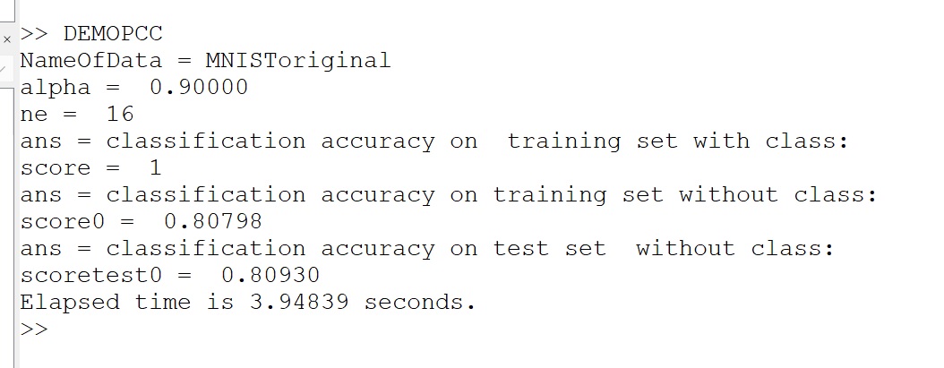
Example of output for MNISToriginal obtained with Octave

The model run by default on MNISToriginal uses 16 principal components and as set $\alpha=0.9$. Accuracy score first reported (acc=1) is for the training set with both feature and class information, the second (acc.= 0.80798) is for the set with the same features but no class provided, and the last is for test set (acc.=0.80930) that has not seen features during training an no class information (see paper). The time reported (3.94839 seconds) is for running the full demo (training+testing of the model), here run on Octave on laptop (Surface Pro 7).

When processing dataset MNIST10, the demo creates some figures but not all work with Octave.

Datasets

MNIST is downloaded from https://github.com/daniel-e/mnist_octave/raw/master/mnist.mat

Datasets wine and australian are downloaded from https://github.com/PouriaZ/GMML

Machine design & data encoding with class (DEC)

In supervised learning, we consider available a dataset $\mathcal{B}=\lbrace(\mathbf{x}^{(i)},\mathbf{y}^{(i)})\rbrace_{i=1,\cdots,N}$ of $N$ observations with $\mathbf{x}\in \mathbb{R}^{d_{\mathbf{x}}}$ denoting the feature vector of dimension $d_{\mathbf{x}}$ and $\mathbf{y}\in \mathbb{R}^{n_c}$ the indicator class vector where $n_c$ is the number of classes. Our approach uses PCA trained on a dataset with training vectors $\mathbf{z}^{(i)}_{\alpha} $
concatenating vectors $((1-\alpha)\mathbf{x}^{(i)} , \alpha\mathbf{y}^{(i)})$

Principal Components are then used for classification even if no class information is available at test time to process a new input $\mathbf{x}$.

Performance

Random permutation training/test sets are used on australian and wine dataset so results change at every run: average over 10 runs is reported here:

Dataset	nb of components $n_e$	alpha $\alpha$	Accuracy (test set)
`MNISToriginal`	16	0.9	0.80930
`MNISToriginal`	618	0.02	0.85410
`australian`	4	0.2	~0.76
`australian`	5	0.2	~0.84
`wine`	4	0.2	~0.88
`wine`	5	0.2	~0.92

Hyper-parameter space

The number of principal components, and the scalar $0<\alpha<1$ are the hyperparameters controlling the model for classification. See below images of accuracy on hyperparameter space for MNIST10 (see paper). These images were created with a for loops computing classification accuracy on a grid defined on the hyperparameter space (code not provided).

Bibtex

@techreport{Dahyot_PCC2022,
   author = {Dahyot, Rozenn},
   keywords = {Supervised Learning, PCA, classification, metric learning, deep learning, class encoding},
  abstract={We propose to directly compute classification estimates
by learning features encoded with their class scores. 
Our resulting model has a encoder-decoder structure suitable for supervised learning, it is computationally efficient and performs well for classification on several datasets.},
 title = {Principal Component Classification},
  publisher = {arXiv},
  year = {2022},
   doi = {10.48550/ARXIV.2210.12746},
  url = {https://arxiv.org/pdf/2210.12746.pdf},
}