In this project, we try to identify how trends have changed for 'automation' across decades, by analyzing The New York Times articles from 1950 to 2021. We also try to identify topics related to 'automation' that managed to consistently get media attention over the decades. We use a variety of approaches and techniques for data cleaning and standardization, and also use packages such as Gensim, spaCy, NLTK, BERTopic etc. to complete the analysis.
The objective can be classified into two:
- Understand the trend around 'automation' using co-occurence of words.
- Understand how topics related to 'automation' have changed across decades using topic modeling.
The implemntation can broady be classified into the following stages:
- Creating the raw layer from source
- Cleaning the data
- Transforming the data
- Analyze the data
- Trend for Automation
- Trend for topics related to Automation
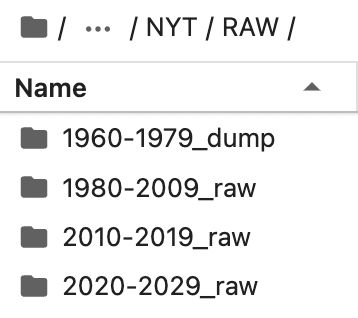
The source of data is from the The New York Times website. All the data for the raw layer reside as text files. We use ProQuest to get the news articles realted to 'automation' as text files. We have images of articles for the years 1950 to 1980, and text transcripts for the articles written after 1980. ProQuest uses an image to text tool to retrieve the articles from the images and return a text file. ProQuest also genereates a metadata file for the articles holding information like Publication info, Publication year, Publication subject, Abstract, Links, Location, People, Place of publication, etc. Each row of the metadata file holds information about one article. This file can be used to categorize the text files as needed. Sometimes, the image to text fails, leading to a mismatch in the number of rows in the metadata file and the actual number of files. An example of a text file generated by ProQuest for articles before 1980 can be seen here, and another example of an article written after 1980 can be seen here. The folder structure for the raw layer is shown below:
The first step involved in data cleaning is to categorize the articles based on the decade it was written. There are a few approaches taken here:
- 1950-1959: No cleaning was required on the articles written during this decade.
- 1960-1979: We use the metadata file generated by ProQuest to identify the files which falls into the 1960-1969 and 1970-1979 decades.
- 1980-2020: Things get a bit more complicated here as the text files generated by ProQuest holds not only the content of the article, but also other metadata. Since the text files follow a particular structure, we use the rules of the structure to our advantage. By identifying the beginnnng and ending of the 'full text' section, we are able to extract just the articles from these files. We also apply the same logic to extract the 'publication year' from the text files, helping us categorize the article based on the decade. We also check if there are any outliers using the same logic.
- 2010-2029: We use the rules used for 1980-2020 to identlify the 'publication year' from the text files, and categorize the article based on the decade. We also check if there are any outliers using the same logic.
- 1950-1959: We encountered some outliers while processing 2010-2019. Upon further inspection, these turned out to be files from 2009. We manually move them to the appropriate folder.
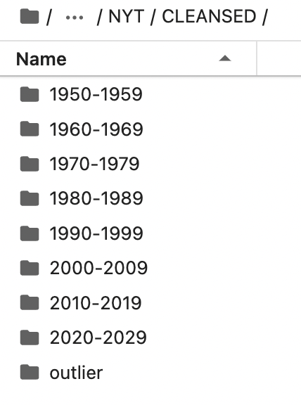
The code for this layer is available here. The folder structure for the cleaned layer is shown below:
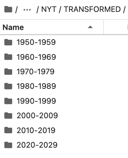
This is the final layer before starting the analysis. We apply a variety of rules in this layer to prepare the data for subsequent layers. First, we remove stopwords, prepositions, punctuations, pronouns and common words from all the articles. The folder structure after this has been applied on the cleaned layer looks like:
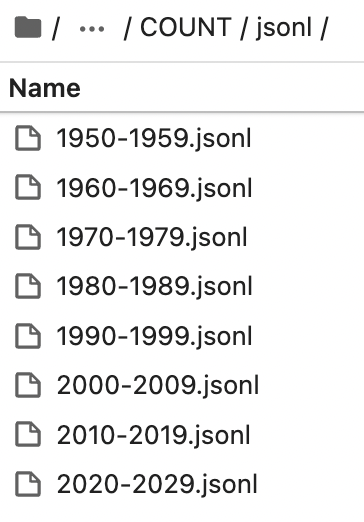
Next, we create unigrams, bigrams and trigrams for each article. We also get the count of each unigram, bigram and trigram generated per article, and format the results into a JSON of format:
[
    ('id', identifier),
    ('outputFormat', ['unigram', 'bigram', 'trigram', 'fullText']),
    ('wordCount', wordCount),
    ('fullText', fullText),
    ('unigramCount', unigramCount),
    ('bigramCount', bigramCount),
    ('trigramCount', trigramCount)
]
Finally, we save the generated JSONs as JSONL files, and do some validation to make sure we have not lost any articles between the cleaned and transformed layers. The code for this layer is available here.
The approach towards the analysis can be split into two methodologies depending on our objective:
To understand how the trends have changed for 'automation' across decades, we look at the frequency of occurence for the word 'automation' in the articles through 3 different persepetives.
Aims to answer how many times the word automation occured as a unigram, bigram or trigram in the corpus for each decade, on a file level. The code for this approach is available here, and the result can be found here.
Aims to answer how many times a bigram or trigram was present in the corpus for each decade, on a word level. The code for this approach is available here, and the result can be found here.
Aims to answer how many times a bigram or trigram was present in the corpus for each decade, on a word level, after lemmatization. The code for this approach is available here, and the result can be found here.
We also build a visualization on top of the results of Persepctive 3 to get a better sense of the distrbution of the top 50 words in the corpus across decades. The code used to build the visualization is available here, and the actual visualization can be accessed here.
We use different topic modeling techniques to find dominant topics in each decade, and also perfrom dynamic topic modeling to capture the evolution of topics. The approaches taken are:
- Decade wise topic modeling using LDA
- Decade wise topic modeling using BERTopic
- Dynamic Topic Modeling (DTM) using LDA Sequence Model
- Dynamic Topic Modeling (DTM) using BERTopic - DTM
The code for these sections are well commented, so I am not discussing them further. You can view and download the code here and, the results as visualizations here.
In this section, we will discuss the results of the analysis: TBD
| Item | Link |
|---|---|
| LDA | https://radimrehurek.com/gensim/models/ldamodel.html |
| LDASeq | https://radimrehurek.com/gensim/models/ldaseqmodel.html |
| BERTopic | https://github.com/MaartenGr/BERTopic/ |
| BERTopic-DTM | https://github.com/MaartenGr/BERTopic/#dynamic-topic-modeling |
| NLTK | https://www.nltk.org/ |
| Gensim | https://radimrehurek.com/gensim/ |
| spaCy | https://spacy.io/ |
| Plotly | https://plotly.com/ |
| Pandas | https://pandas.pydata.org/ |
| Numpy | https://numpy.org/ |
| Haystack | https://haystack.deepset.ai/overview/intro |
| scikit-learn | https://scikit-learn.org/stable/index.html |
| pyLDAvis | https://github.com/bmabey/pyLDAvis |
| The New York Times | https://www.nytimes.com/ |
| ProQuest | https://www.proquest.com/ |


